The EM algorithm for me is one of those things that I feel I should know back to front, since it’s a pretty foundational algorithm in probabilistic ML. Unfortunately though I’ve never actually used it explicitly in a model I have built, despite reading about it in various textbooks, so I never properly got to grips with it. If you feel the same way, then hopefully this question will help. It’s from the new Murphy book, which is a fantastic reference. So much for sticking to a problem a week, hopefully it won’t be such a long gap to the next one!
Problem
Derive the EM equations for fitting a mixture of linear regression experts.
Source: Probabilistic machine learning: an introduction by Kevin P. Murphy, Ex. 11.6
Solution
We can fine the specification of the mixture of linear experts model in section 13.6.2.1 of the book. For input data \( \{(x_n, y_n)\}^{N}_{n=1} \) with \( x_n \in \mathbb{R}^D \) model consists of a set of \( K \) linear models (called the experts), with weights \( w_{k}\in\mathbb R^{D} \) with each linear model having a Gaussian likelihood, with noise variance \( \sigma^2_k\). Additionally, we have a \( K \)-class logistic regression model, with weights \( W\in\mathbb{R}^{K\times D} \), which outputs the probability that each expert is responsible for a particular data point. This model is written as,
\begin{align} p(y|x_n,z=k,\theta)&=\mathcal{N}(y|w_{k}^{\mathsf{T}}x,\sigma_{k}^{2})\\\ p(z=k|x,\theta)&={\mathrm{Cat}}(z|{\mathrm{softmax}}_{k}(\mathrm{V}x) \end{align}
where \( \mathrm{Cat} \) is the categorical distribution and \( \theta=(W, V, \{\sigma_k\}^{K}_{k=1}) \) is our set of model parameters (in this case we assume \( K \) is known, or selected by some other method like cross validation). The aim is to use EM to fit this model by finding \( \theta \). Before getting into that, it’s perhaps helpful to look at the type of problem this model might be useful for.

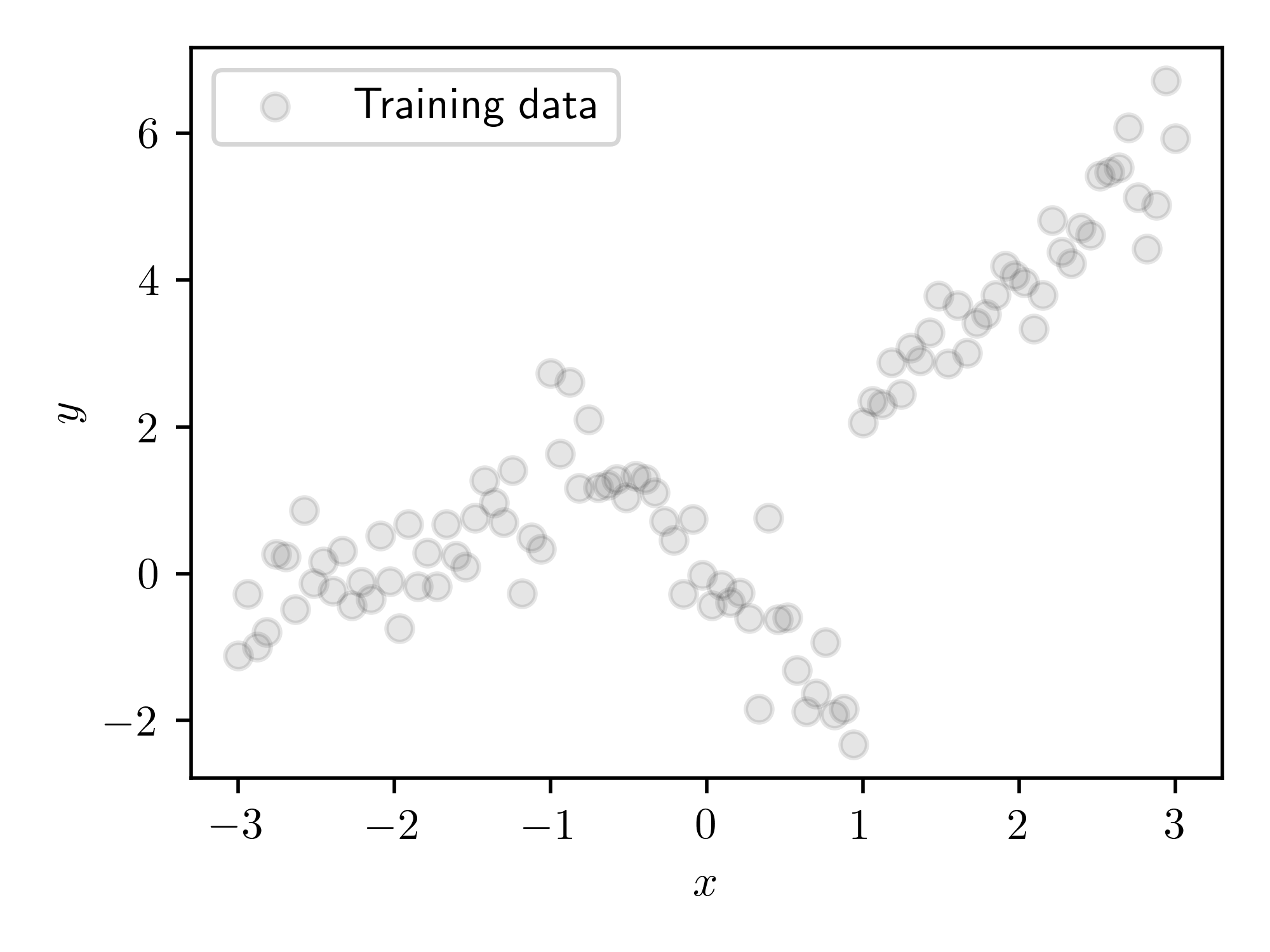
Some training data.
This is some data from a piecewise linear model, with 3 sections, with Gaussian noise added to it. We would hope that a mixture of linear experts model would be able to fit this data well, by assigning a different expert (i.e. linear model) to each of the distinct sections.
Now for inference. Recall that the point of the EM algorithm is to compute the maximum likelihood estimate of the model parameters, whilst marginalising out any latent variables. In this case the latent variables are the expert assignments for each data point, i.e. which expert is responsible for each data point. To do this, we alternate between two steps the E-step and the M-step, until we reach some sort of convergence:
- In the E-step, we compute the distribution of the latent variables (expert assignments) given the data and parameters, \( p(z_n=k| y_n,x_n, \theta) \). In our case this is is tractable, if it’s not then you can use an approximating distribution, in which case the method becomes variational EM.
- In the M-step, we compute a quantity called the expected complete data log likelihood. This is the expected joint log probability of the data and latent variables, with respect to the distribution over the latent variables computed in the E-step, which we write as \( \ell(\theta)=\sum_{n}\mathbb{E}_{q_{n}(z_{n})}\left[\log p(y_{n},z_{n}|\theta)\right] \) with \( q(z_n)=p(z_n=k| y_n,x_n, \theta) \). We maximise this with respect to \( \theta \), i.e compute \( \theta^*=\mathrm{argmax}[l(\theta)] \). We then set \( \theta=\theta^* \) and repeat the E-step.
We repeat this until the optimum of value in the M-step converges. For more info, see section 8.7 of the Murphy book. Now we can try to compute the required quantities for each step for the linear experts model.
We can compute the distribution over the latent variables given the data in the E-step using Bayes rule,
$$ p(z_n=k| y_n,x_n, \theta) = \frac{p(y_n | z_n=k, x_n, \theta)p(z_n=k| x_n, \theta)}{p(y_n|x_n, \theta)} $$where \( p(y_n|x_n, \theta)=\sum^{K}_{k'=1} p(y_n | z_n=k', x_n, \theta)p(z_n=k'| x_n, \theta) \). This is tractable, we just combine the terms given in the specification of the model. Easy! Now for the M-step, which is slightly more involved.
For the M-step we need to compute \( \sum_n\mathbb{E}\_{q_{n}(z_{n})}\left[\log p(y_{n},z_{n}|\theta)\right] \) with \( q_(z_n)=p(z_n=k| y_n,x_n, \theta) \). The log joint is given by, \begin{align} \log p(y_{n},z_{n}|\theta) &= \log p(y_{n}|z_{n},\theta)p(z_{n}|\theta) \\\ &= \log \prod_k\left[\mathcal{N}(y_n|w_{k}^{\mathsf{T}}x_n,\sigma_{k}^{2})\right]^{z_{nk}} + \log\prod_k\left[\frac{e^{v_{k}^\top x_n}}{\sum_{k’}e^{v_{k’}^\top x_n }}\right]^{z_{nk}} \\\ &=\sum_k {z_{nk}\log \left[\mathcal{N}(y|w_{k}^{\mathsf{T}}x,\sigma_{k}^{2})\right]} + \sum_k{z_{nk}}\log\left[\frac{e^{v_{k}^\top x_n}}{\sum_{k’}e^{v_{k’}^\top x_n }}\right] \end{align} where \( z_{nk} \) is an indicator variable which is \( 1 \) when \( z_n=k \) and \( 0 \) otherwise. We can the compute the M-step obejective as,
$$ \begin{align} \ell(\theta)&=\sum_n\mathbb{E}_{q_{n}(z_{n})}\left[\log p(y_{n},z_{n}|\theta)\right]\\ &= \mathbb{E}_{q_{n}(z_{n})}\left[\sum_{nk} {z_{nk}\log \left[\mathcal{N}(y|w_{k}^{\mathsf{T}}x,\sigma_{k}^{2})\right]} + \sum_{nk}{z_{nk}}\log\left[\frac{e^{v_{k}^\top x_n}}{\sum_{k'}e^{v_{k'}^\top x_n }}\right]\right] \\ &= \sum_{nk} {\mathbb{E}_{q_{n}(z_{n})}[z_{nk}]\log \left[\mathcal{N}(y|w_{k}^{\mathsf{T}}x,\sigma_{k}^{2})\right]} + \sum_{nk}{\mathbb{E}_{q_{n}(z_{n})}[z_{nk}]}\log\left[\frac{e^{v_{k}^\top x_n}}{\sum_{k'}e^{v_{k'}^\top x_n }}\right] \end{align} $$where \( \mathbb{E}_{q_{n}(z_{n})}[z_{nk}]= p(z_n=k| y_n,x_n, \theta) \) are exactly the values computed in the E-step. We are now able to compute \( \ell(\theta) \), but we also need to optimise it. I think would be possible to compute the optimum with respect to the regression weights and variances exactly, using the formalism of weighted least squares, but if you’re lazy like me, you can just do simple gradient descent on the parameters. You’d have do this for the logistic weights anyway, since they can’t be computed in closed form, so it’s easier to just do this for everything.
Now we have both steps we can do inference. I implemented this using jax, which made the the optimisation for the M-step very easy. You can find the very shoddily written code in this gist.

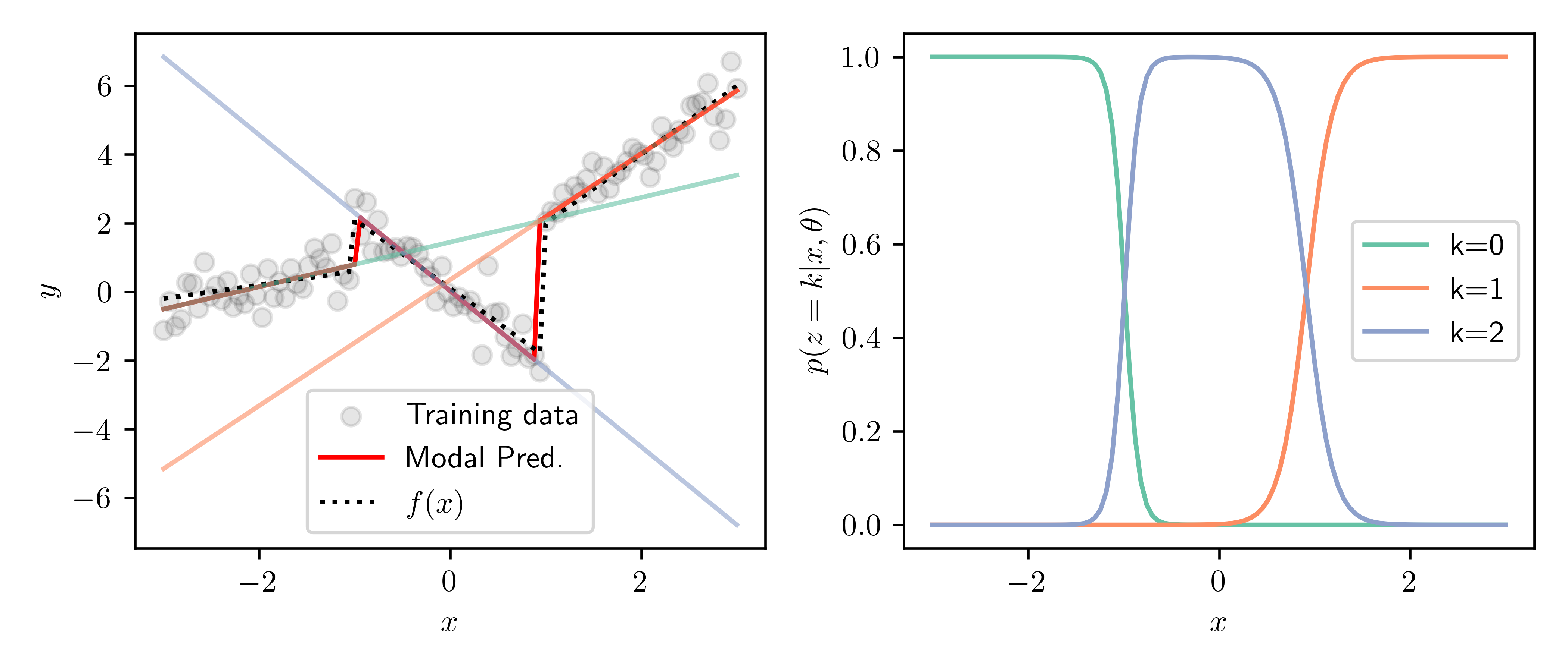
Results of inference.
Above are the results after 20 EM iterations. The left panel shows the training data and true function, along with the predictions of each of the \( K=3 \) experts. Shown in red is the modal prediction, i.e. the prediction of the most likely expert for each point. The right panel shows the responsibilities of each expert for over the domain. We can see the transitions between experts nicely match the discontinuities in the piecewise function, and we are able to recover the true function well.