Or, understanding the Cradle-1 pipeline.
Lead optimisation is the step in drug design where you take a molecule that sort of works and try to make it actually work, and it’s arguably the step where most real-world design campaigns succeed or die. Due to the influence of a couple of my pals, I have recently become interested in using machine learning to do lead optimisation for proteins. Said pals have been kind enough to indulge my extremely beginner level questioning over the few weeks. I’m going to use this post to share what they have taught me, in the hope it might in turn help you understand a bit more about this fascinating area. Like any field, there are some established principles that are never spelled out explicitly in the literature, which can make it confusing for newcomers. We’re going to try to understand how we could actually build a real system for lead optimisation but studying one that has been shown to work well in real life.
Firstly, before we get into it, what actually is a protein? I think to answer this in full we would need multiple textbooks/degrees. Since basically all of my knowledge of biology comes from one read through of Philip Ball’s How Life Works I am convinced the answer to any question about biology is arbitrarily arcane and complex, so for now it will suffice to say that proteins are a class of molecule which are an integral part of basically all the processes that sustain life. Proteins are chains of smaller molecules called amino acids of which there are 20 different types.1 As such we can represent a protein as a string of characters, with a character standing for a different amino acid, using all the letters of the alphabet apart from BJOUXZ.2 For example, we can write myoglobin, a protein responsible for shuttling oxygen around our cells, as:
MGLSDGEWQLVLNVWGKVEADIPGHGQEVLIRLFKGHPETLEKFDKFKHLKSEDEMKASEDLKKHGATVLTALGGILKKKGHHEAEIKPLAQSHATKHKIPVKYLEFISECIIQVLQSKHPGDFGADAQGAMNKALELFRKDMASNYKELGFQG
For certain combinations of amino acids, this chain folds up into a fixed shape, which allows that protein to perform a function. Predicting the shape of the fold from its sequence is, to put it mildly, highly non-trivial, and is the problem the AlphaFold-2 model “solved” to some extent to win the Nobel Prize in Chemistry. It is important to understand that there are many possible combinations of amino acids, and most of them will not fold into a regular, predictable shape, and do not do anything useful.3 The folded myoglobin looks something like this:
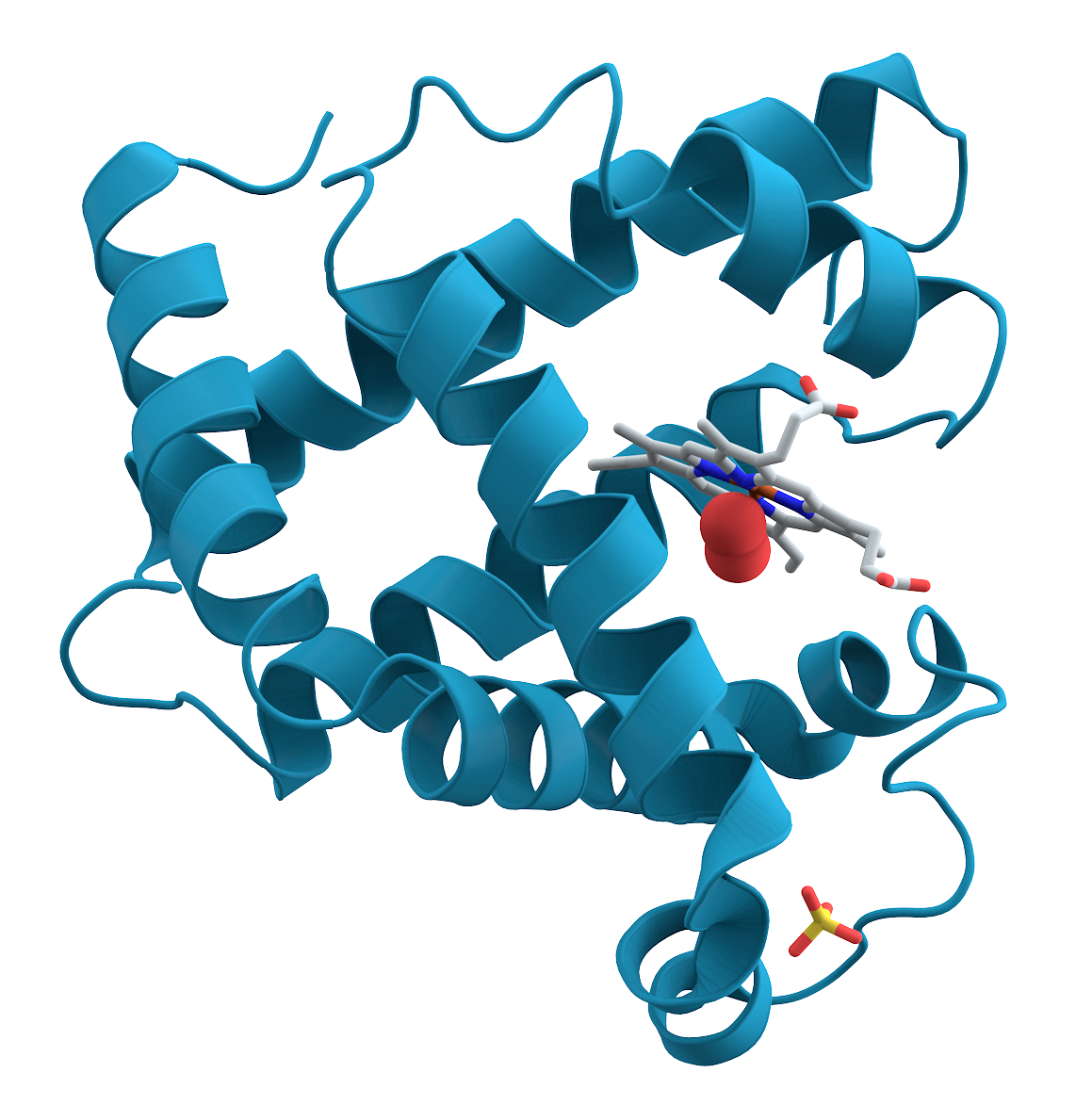
The structure of myoglobin. Public domain, via Wikimedia Commons.
Typically proteins consist of about 300 amino acids, but the largest, which is comically named PKZILLA, contains upwards of 40,000, and they can be as small as 20. There are estimated to be between 80,000 and 400,000 different proteins that perform functions in human cells. Note that when the amino acids are bonded to form the protein each one is known as a residue. The proteins that exist in nature are the result of evolution. Because of this we can group proteins into families which have some similarity to each other; within these families a large proportion of the sequence representing each protein will be the same. So now we very roughly know what a protein is, what is protein design?
The ultimate goal of protein design4 is to generate new molecules that perform a certain function. This function can range from catalysing a specific chemical reaction to binding to a disease causing molecule. Lead optimisation is one of the most important steps in the design process. We assume that we have an existing template molecule that is functional to some extent, but is not sufficient for our ultimate goal. This molecule might have been the result of a previous failed design campaign, generated de novo (i.e. from scratch) by some other model, or chosen from nature. The process of lead optimisation involves proposing changes to this initial molecule with the ultimate goal of improving its properties for the task at hand. In practice, the function of the protein for this task can rarely be summarised by a single number and we usually care about several properties at once and these can trade off against each other. For simplicity, we’ll mostly talk as if we’re optimising a single property in this post, but keep in mind that the real picture is multi-objective.
The process of lead optimisation proceeds by proposing a set of candidate changes, testing them in the lab, and then proposing more changes after integrating the results of the lab tests. The way this traditionally worked was by using directed evolution, which essentially involves introducing random mutations, testing them and keeping the ones that improve function and mutating them further in a loop until we get to sufficient performance. Given that we have massive databases of proteins, and the awesome power of deep learning, these days we can probably do better.5 And indeed some people have!
Cradle is a bio-tech startup that sells a system for ML-based protein lead optimisation. They’re somewhat unusual for a bio-ML company in operating their own wet lab, which they claim gives them a unique ability to keep the loop between model suggestions and experimental feedback tight. Their system seems to be a market leader, and they are working with a number of the world’s largest pharmaceutical companies (e.g. Novo Nordisk, Bayer, J&J). They have demonstrated impressive results across a number of different contexts. Cradle recently published a white-paper, describing how their system works at a high level. Here it is:
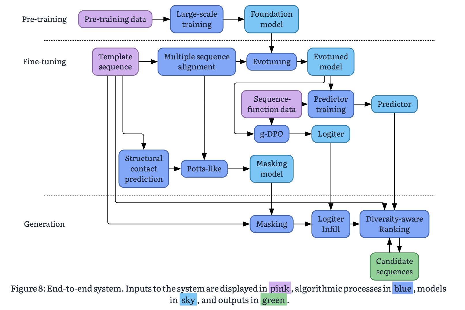
Lifted from the Cradle whitepaper.
The base model
There are a lot of models shown on the big diagram, a somewhat scary number, but actually most of them are tweaked versions of the same fundamental backbone: a transformer-based protein language model. If we can understand that we can go a long way to understanding the pipeline. The standard language modelling paradigm (that powers Claude, ChatGPT etc) is fundamentally based on next-token prediction; a token is a word, or part of a word, and we task models to predict the next word given proceeding context. Typically there are 10,000s of possible tokens corresponding to the large number of words in our vocabulary. We can apply this paradigm directly to modelling proteins by substituting our large vocabulary of words for our 20 different types of amino acids, since proteins are just sequences of these. To train our model, we take a dataset of protein sequences, and cover up some of the residues, and get the model to predict which amino acid was in that position based on the others around it. We can do this either by covering up the end of the sequence in the same way we would do in a standard language model, which is known as next-token prediction, or by covering up a residue in the middle of the sequence which is known as masked language modelling. The base model in the Cradle pipeline takes the latter approach, so we will focus on that. The problem essentially looks something like this:
 M K T A [?] G L S E R ...
          |
    L  ██████ 0.42
    V  ███    0.28
    I  █      0.15
    ...
The base model produces a distribution of probabilities over amino acids likely to fill the missing position. The first step of the Cradle pipeline is to take this model structure, and train it on a dataset of tens of millions of natural proteins. This is what is happening at the top of the diagram in the section labelled pre-training. The idea here is to produce a model that has learned something about the features of natural proteins. Such a model is actually useful in its own right because it gives us a way of understanding if certain edits to a protein are likely to ruin it, that is to say to cause it to become disordered or not expressed or whatever. The model gives us suggestions for residues we could place at a specific position to make a natural protein. Say we mask a G in a known protein and the model predicts that that position was 0.001% likely to be a W but 40% likely to be a V, we can conclude that the protein with the W is unlikely to be functional. The model is saying that it has never seen a protein that looks like that in nature, and we believe that since many millions of years of evolution has produced the set of proteins that exist, those that don’t are unlikely to be useful. We should note that this is not something we know for sure to be true. It is possible that there may be proteins that are functional that are very different from natural ones; these are going to be very difficult to model with machine learning because, by definition, we have very little data about them.
Now we have an understanding of what the base model does (it predicts how “natural” specific edits to individual amino acids are) we have covered the top three boxes. We can now move on to the next section, which has a lot more going on.
Evotuning
The space of natural proteins is very large and diverse. The process of lead optimisation is about improving the function of a protein for a specific use case. When using a model trained on the space of all proteins, the model is unaware of the specifics of the function we are trying to optimise for; it is too general. It is possible for the base model to make suggestions that are natural, but would be totally unhelpful for our use case. How can we push the model to make more relevant suggestions? The answer is to use fine-tuning.
Fine-tuning is the process of adapting a more general model to perform well on a more specific task by training it on a representative set of data from that task. In lead optimisation, we start with a single template protein which already functions to some extent, and we want to improve this function further. We want to form a fine-tuning task to push the model to suggest proteins that are likely to be functional. We can do this by finding all the natural proteins that are likely to be evolutionarily related to the template, and training the model on them. The idea is that if they are evolutionarily related, they likely share some function. We want the model to “focus” on this area of the full protein space.
We form the set of evolutionarily related proteins by using something called a Multiple Sequence Alignment (MSA). Understanding MSAs fully would be its own whole thing, but the rough idea has two parts: first, we search a huge database of protein sequences for ones that are statistically likely to share a common ancestor with our template (these are called homologs). Then we align them, i.e. line them up residue by residue so that positions playing the same structural or functional role sit on top of each other. This is complex because not all of the homologs will necessarily be the same length, so we need to account for insertions and deletions. Once we do this we can glean some extra information about the sequence. I’ve tried to illustrate this with some more ASCII below.
Query    : M K T A Y G L S E R N

Hit 1    : M K S A Y G L T E R N    (91% similar)
Hit 2    : L K T A Y G L S D R N    (81% similar)
Hit 3    : M R T A Y G I S E K N    (73% similar)
           ─────────────────────
Conserv. : x x x ✔ ✔ ✔ x x x x ✔
In this example, the database returns 3 similar sequences, but in reality it would be thousands. We can see that there are a number of positions (4, 5, 6 and 11) where all the proteins share the same amino acid, i.e. they are conserved. We can be fairly sure, then, that in any protein we suggest for further testing, these positions should also be the same. In real proteins, it isn’t just particular positions that are conserved but motifs: sequences of amino acids like AYG in this example.
Once we have our MSA for the template, we take our pre-trained model and train it further on those sequences. This pushes the model to make suggestions that are consistent with the evolutionary context of the protein in question, which we hope will mean the model’s suggestions are more likely to be functional. This process is called evolutionary fine-tuning, or evotuning. So we now have an idea of what’s going on in the top row of the fine-tuning section. We should note here that there is another arrow from the MSA box, to “Potts-like”. We’ll get to this in the next post, but the MSA information is also useful for generation because it tells us something about which positions are likely to be important to the structure of the protein.
What about the lab?
When I introduced the lead optimisation problem, one of the key steps was testing the function of the proteins in the lab. The ultimate goal of the whole process is to optimise these measurements, so how do we incorporate this information into the process? In this section we’ll discuss how we can use the sequence-measurement pairs to push our model to suggest proteins that are likely to score better, and how we can adapt the model to actually predict the likely score of future candidates for testing.
First we need to get at least a surface level understanding of what these measurements actually look like. In biology, lab tests like this, where we are measuring some aspect of the function of some substance (in this case, a protein) are called assays. What these assays measure is very dependent on what function we are optimising for and, as mentioned earlier, a single assay run often returns several measurements at once, since we typically care about multiple properties simultaneously. It’s important to realise that the measurement values are pretty much always an imperfect proxy for the true function we are interested in. For instance, we might measure how a protein performs against a single purified target in a test tube, when what we really care about is how it behaves in the messy environment of a living cell. The data we get out typically looks something like this:
Sequence                          Activity   Stability
─────────────────────────────────────────────────────
M K T A Y G L S E R N ...          0.82       54.1
M K T A Y G L T E R N ...          0.79       53.8
M K S A Y G L S E R N ...          0.91       52.4
M R T A Y G L S E R N ...          0.44       55.0
M K T A Y G I S E R N ...          0.88       51.9
M K T A Y G L S D R N ...          0.71       53.2
There are many different kinds of assay. Often assays are performed in batches, where there is a plate with multiple wells laid out in a grid and a different protein is tested in each well. This means that at each round of testing we obtain a set of new data points. In the Cradle setup this seems to be 96 most of the time. Typically in machine learning we assume that points in our dataset are statistically independent from one another. This assumption can be violated in the context of batched assay measurements because there are quirks of the measurement process that affect all the measurements in the grid simultaneously. Additionally, weird stuff can happen at the edges of the grid which make those measurements less reliable. Any model we create needs to be robust to these batch effects; we won’t discuss them further here but it’s important to consider when building a system like this.
Pushing preferences
Now we know roughly what the “sequence-function” box corresponds to, we can see that this leads to two downstream models. Let’s tackle the more arcane “g-DPO” first. About a year ago in my office DPO seemed to be basically the only thing anyone was talking about. These days things have cooled off a bit and it’s been cemented as one of the key methodologies powering LLM post-training (the bit where we turn the LLM from fancy autocorrect to all-powerful agent). DPO stands for direct preference optimisation; there are about a million blog posts explaining it way better than I could (here is a mathsy one and a less mathsy one), so I’ll spare you. The basic idea in the LLM context is that we have some preference data consisting of prompts (e.g. “Is B a standard amino acid?”) and a pair of possible responses, one good (e.g. “No”) and one bad (e.g. “Yes, and you’re a loser”). We want to try to push the model to give us more good responses and fewer bad ones. DPO gives us an efficient way to do this without having to introduce extra scoring models and other fancy reinforcement learning things, which was the way this was done before.
In our context we want to push the model to generate more proteins that have higher function values, as measured by the assay, and fewer ones with lower values. The format of the assay data doesn’t really match up with the pair of completions in the original DPO setup. One way we can massage it a bit to get these pairs is by setting a threshold for the assay measurements: if the measurement is above the threshold it’s “good”, and if not, it’s “bad”. How we actually pair sequences up is much less clear than in the language case however, and it all gets a bit messy. All in all trying to directly apply DPO here is a bit square peg round hole, so the Cradle people introduced a variant called grouped DPO (“g-DPO”). In g-DPO we group proteins into clusters with similar sequences, and then we form pairs from within the group. The idea is that if we compare sequences that only differ by a few positions (as they do within the group) the model learns how subtle changes affect the protein function; when comparing very different sequences the model learns more obvious differences.
We take our sequence-function data and apply the g-DPO method to further train the evotuned model from the previous step. At this stage, we ideally have a model that is really good at suggesting changes to our template sequence that will result in a more functional protein. This model is called the “logiter”6 on the diagram. Now onto the next box!
Forecasting function
We have one more model to tackle before we can run generation: the “predictor”. The point of the predictor is pretty much what it says on the tin: we want to predict the assay value(s) (the function) from the sequence. We’ll get into the details next time, but we can use this predictor to filter the suggestions of our logiter and prioritise what to send for testing.
A good model for protein sequences should be able to capitalise on meaningful features of the sequence and use them to make predictions. We (hopefully) already have a good model for protein sequences: the evotuned model. This is not a model for predicting function, but instead for predicting the sequence itself. In order to be good at that however, the model must learn useful representations of the sequences. Inside the transformer, each position in the sequence is associated with a vector of numbers that gets progressively refined as it passes through the layers, ending up as a sort of summary of what that residue is doing in the context of the whole protein. These vectors are what we mean by representations, and the final amino acid prediction is just a simple operation applied on top of them.
The structure of this model allows us to access the representations it has learned, and use them for other purposes. This is the approach we take to build the predictor. We feed the learned representations from the evotuned model into a simple model that uses them to predict the assay values. We call this simple model a regression head because we attach it to the top of our model. The intuition is that if we can predict the residue at different positions in the sequence (as we do with the evotuned model) accurately, then we must have learned some useful information about the sequence. This information will also be useful for predicting whether the sequence is functional. The beauty is that most of the work has already been done; we just need to adapt this information a bit for our new purpose.
Wrapping up (for now)
OK, so after all that, what are we left with? We now have two key models that will allow us to stride forth and generate some proteins: the logiter and the predictor. In generation, we’ll use the former to make suggestions, and the latter to rate them. There is one quite important thing we’ve skirted around up to now. The logiter gives us a prediction for which amino acid is likely to work well at a given position, but it assumes that we already know which position we are interested in modifying. Determining which positions to modify is by no means trivial, and is the responsibility of the “Masking model”, which we’ll get to next time.
Thanks for bearing with me, and I look forward to seeing you in part 2 for more protein fun!
And thanks very much to David Miller for reviewing this post and highlighting a number of oversights.
-
There are actually more, but the other ones are too rare to bother caring about very much. ↩︎
-
Which sounds kind of like a French word, or a club they’d go to on Geordie Shore ↩︎
-
This is a massive simplification and is not really true. Proteins that don’t fold into a regular shape are called intrinsically disordered and they actually can do important things, but this is a very active area of research. People are also trying to use ML to design these things, but this is a bit of a different problem and so we won’t discuss it further here. ↩︎
-
I think technically lead optimisation, where we are modifying an existing protein to improve its function rather than creating something new, is known more as protein engineering in the field. ↩︎
-
It should be noted that although it sounds simple, getting directed evolution to work well for real problems was a huge achievement and resulted in half a Nobel Prize for Frances Arnold. ↩︎
-
It’s called this because it outputs logits which are the raw numerical scores a neural network spits out for each option (in our case, each amino acid) before they’re normalised into probabilities that sum to 1. ↩︎