This is nothing to be proud of, but I have never really studied optimisation in depth. Oh sure, I know my Adam from my AdaGrad and I even used L-BFGS one time, but when people start talking about dual spaces and convergence for continuous functions, I tend to glaze over a bit. For some reason I think in my head a lot of it seemed a bit old fashioned, whatever that means; why do I need to learn about optimising constrained convex functions in the gradient-descent-for-everything-wait-actually-just-use-a-pre-trained-model era? Isn’t that what they used to, like, make the cheapest possible diet? Boring!
Well, today on the blog, I’d like to talk a bit about my optimisation blind spot in the context of an interesting problem I have been working on related to protein binder design. The first way you think to do something is rarely the best; here we’re going to discuss a concrete example of that. If you, like me, are not an optimisation expert, then I hope you’ll learn something useful from this post. If you are, then feel free to have a good old laugh at my ignorance!
Setup
Ok so what’s the setup? Let’s say we have a categorical probability distribution with categories where the probability of each category is given by the vector . There are some constraints on for it to be valid:
- the probabilities must be normalised: ,
- and, the probabilities must be greater than 0: .
We have a non-convex function which takes in our probability vector, and spits out a real number. We want to find the that minimises this function . In our setup, we will assume we can compute the gradient , but evaluation of the gradient, and indeed the function itself, is computationally expensive.
Protein related aside
This is a simplified version of the problem of hallucination for de-novo binder design where represents a distribution over amino acids, and is a folding model, like Alphafold which takes a sequence of of these amino acid distributions, called a position specific scoring matrix (PSSM), as input. We want to find the sequence that gives the best fold (according to some metric like ipSAE). In this case the input to is now a matrix where each column is a probability vector.
A first attempt
When seeing a problem like this, where we need to optimise something with constraints, my first instinct is to try and re-parameterise the problem so that I don’t have to worry about them, and we can just use all the “normal” methods. We basically want to rewrite as a function of some other parameters with no constraints, then we can just optimise those. In this case, we can write
where we call the logits. Note that for any , the output is guaranteed to be a valid probability vector obeying the constraints we set out earlier. Perfect! Problem solved! Now we can just find by taking gradients w.r.t. and running some gradient descent method, and get . This all makes sense, and would have been case closed for me in the past, but it turns out there are other ways, and those ways are interesting!
The simplex
Let’s take a step back and think a bit more about the structure of this problem. It turns out there is a special name for the space of ’s that obey the constraints set out at the start: the probability simplex , so we can write . The probability simplex is the dimensional region of space where both non-negativity and normalisation are satisfied. Let’s take the concrete example of with categories . The 2-simplex is a triangular region oriented perpendicular to the direction, it looks something like this:
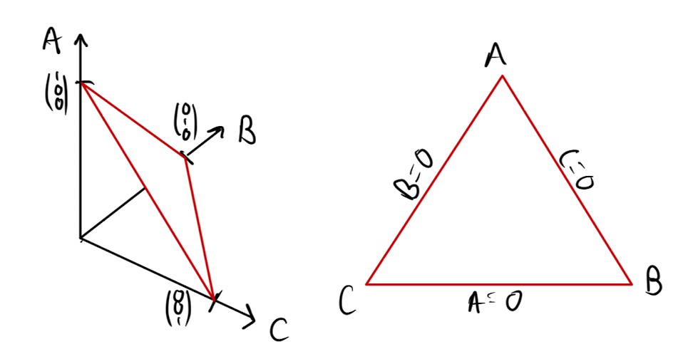
2-simplex in 3D and 2D.
On the left we show the region in the full dimensions, and on the right, we show the 2D “top down” view. The vertices of the simplex are the points where we have one category with certainty. On the faces, one of the categories doesn’t contribute (e.g. on the A/C face, B doesn’t contribute). Our optimisation problem boils down to finding the smallest value of that lies on this simplex.
You’re projecting
Let’s think about what happens if we just try the simplest possible thing we can think of: we start at a point on the simplex, take the gradient and try to run a step of gradient descent: . There are approximately four things that can happen:
- We step “above” or “below” the simplex region, which happens if our gradient is not perpendicular to . In this case we would be adding to all the probabilities at once, which isn’t allowed because it breaks normalisation.
- Our gradient is perpendicular to , but we step “outside” the triangular region, which corresponds to one of the coordinates becoming negative.
- We really mess up, and do both 1. and 2.
- We do neither 1. or 2. and stay on the simplex 🥳
So in general, we’re going to end up off the simplex, in an invalid region. It turns out we can actually avoid case 1. pretty easily by just computing the component of the gradient that is perpendicular to , and stepping in that direction. We can do this by subtracting the mean of the gradient components.1 From now on we just assume we always make the gradients centred. This leaves the only problem with applying gradient descent to the raw probabilities as case 2., where we step outside the valid region. Here’s how that might look
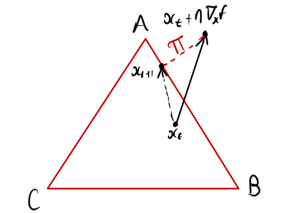
One step of PGD on the 2-simplex.
with the black arrow representing the raw gradient descent step. We need to find a valid point in order to take the next step. To do this we compute the projection of the step onto the simplex, which is to say we find the nearest point on the simplex to the desired raw gradient step. This projection operation is represented by the red dotted arrow, with the final step given by the black dotted arrow. This process is called projected gradient descent (PGD) and is, in a way, conceptually simpler than our initial reparameterisation solution. If we want to optimise just run GD and correct it any time we go wrong. One step of PGD can be written as
where is the projection operator onto the simplex. Computing the projection is actually not trivial, and we won’t go into details here, but there are ways to do it in time by using a couple of cool tricks. You can read about it in this classy ICML paper from ‘08. Basically it’s very fast relative to the cost of computing the gradient.
It’s worth noting a few things that aren’t necessarily intuitive from our simple 2D case above when we scale to higher dimensions. Firstly, as the dimensionality of the simplex increases, the probability we step off the simplex with a gradient step becomes larger and larger; more points inside the simplex are close to an edge. Whenever we step off the simplex, we get projected back onto a face, where at least one coordinate is set to zero. In higher dimensions it becomes increasingly likely we end up projected on lower and lower dimensional faces, resulting in sparser steps. If we run a quick simulation and take a randomly directed step from one of the vertices, then in 2D the probability we step back inside the simplex is , for it’s about , and for it’s essentially 0. Basically what all this amounts to is that PGD in high dimensions has a tendency to produce sparse solutions, which get sparser as optimisation proceeds. This is interesting and useful to bear in mind.
Looking into the mirror
Applying a softmax to get probabilities from unconstrained real numbers is of course a very common operation in machine learning, and so the reparameterisation in the first section feels natural, but it’s worth taking a step back and thinking about how we can justify this. Why not use a different function that maintains non-negativity/normalisation? We could do all sorts of fun things here. We’ve got to remember that since is non-convex, using different transformations is likely going to give us a totally different answer for the optimum, because we’re probably not going to find the global optimum. Because of that our choice of transformation is actually very important. To add some mathematical flesh to this choice, we’re going to need some extra machinery, in this case that’s something that’s intriguingly called mirror descent. If you’re good at maths you can read these lecture notes (chapter 17), which are very clear. I’m going to try to transmit the salient points.
What’s actually going on when we do standard gradient descent? When we take a gradient step, we are making the assumption that the local neighbourhood of our current iterate can be well approximated by a linear function (the first order Taylor approximation). When we take a step we want to minimise this approximation. If we just did that however, we’re going to end up at infinity, because a linear function has no minimum, so we need to make sure we stay in the neighbourhood. We can do this by introducing an additional penalty to our minimisation: the L2 distance from the iterate. So at each step we want to find
If you differentiate this w.r.t. then set it to zero to find the minimum, then you get that
so the optimum for each step gives us standard gradient descent. If you’re switched-on, you might be thinking: wait? Why the L2 norm? What’s the justification for that? Well dear reader, that would be a fair question, and actually the beauty is we can (subject to some rules) choose different penalties here, and generate different algorithms. The class of penalty we can choose from here are called Bregman divergences. For some strictly convex function , the Bregman divergence between points and measures the difference between the value of at the point and the linear approximation of taken at point , so
This is probably much clearer if you check out this handy visualisation (re-drawn by me from the lecture notes):
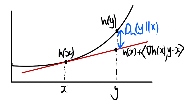
A visualisation of the Bregman divergence for a one dimensional function.
here the Bregman divergence is in blue. If you use then you get the squared L2 distance back. In the general case at each step we’re then trying to solve (dropping constant terms)
Differentiating and setting to zero in the same way, we get that (with a bit of fiddling)
You’re probably wondering what the point of all this is, and also why mirror is in the section title (we’ll get to that), so let’s look at a little motivating example. What if, bear with me here, we use the unnormalised negative entropy function in our Bregman divergence? Well, we get that
where we’ve applied the linearity of the gradient, and the normalisation of the probability vectors. The Bregman divergence = the KL divergence in this case! We can interpret this gradient update as minimising the linear approximation of whilst ensuring the update is close in KL-terms, instead of Euclidean. This is interesting because it means we actually now can’t get negative entries for the probabilities (they would have infinite KL), so one of the simplex constraints is automatically fulfilled. Unfortunately, this step is not automatically normalised. To ensure that it is, we project onto the simplex by finding the point that is closest in terms of KL divergence to our unnormalised vector. This turns out to just be equivalent to dividing by the sum of the vector, i.e. normalisation.
Notice that , so we can interpret the update equation as applying the gradient update from “probability space” to the logits, and then mapping back to probability space with . We can see that this actually gives us a very similar update to our original softmax reparameterisation (with our additional normalisation term is exactly the softmax), but there is one important difference: we are using the gradient in probability space, instead of logit space. This means that the updates differ by a factor of the Jacobian of the softmax, i.e.
We can see why this is an issue if we look at a case near a vertex, say with small then we end up with a Jacobian with each entry . This means that the gradient vanishes and so the optimisation trajectory can get “stuck” near a vertex. Bad stuff!
Ok so we’ve established a more theoretically well grounded update rule related to the softmax reparametrisation, but with a crucial difference in the specific gradient we use. Turns out the theory actually goes much deeper. I won’t go into too much detail here, because it’s giving me unpleasant flashbacks to failing to understand field theory in my undergraduate physics lectures, but the point is that if you think about it, it’s quite strange that we are adding the gradient vector to the parameter vector. If we apply a bit of the ol’ dimensional analysis then has units and has units , so the two can’t be added unless the step size secretly carries units of to convert between them, when it should in fact be dimensionless. This is because the gradient is actually not a vector, but a “covector”2 that lives in a different space, called the “dual space” to the “primal space” where the parameter lives. Basically the idea is that we can view the gradient as a linear function which when applied to a vector (with an inner product) gives us the rate of change in that direction. All such linear functions make up the dual space.
It turns out this esoteric theory can actually help us to understand the update equation above. If we call the mirror map, then maps us to the dual space, where we apply the gradient update, and then maps the update back to the primal space. The inverse mapping may put us outside the constraint region, so we apply a final projection to get the update. We can see from my lovely diagram why it’s called mirror descent. We are descending in the dual space, which “mirrors” our real space.
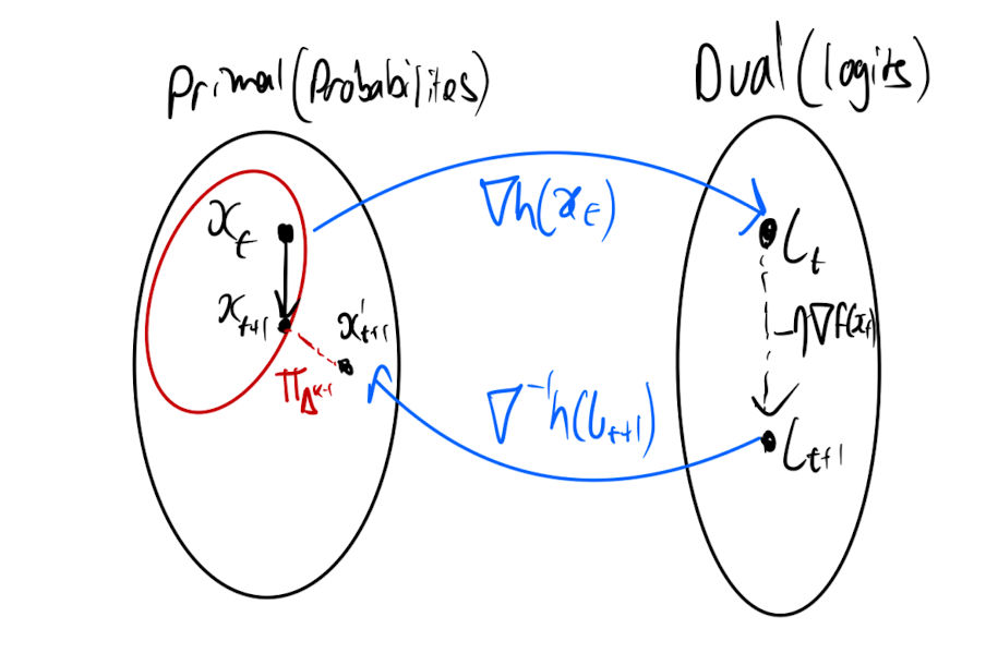
One step of mirror descent.
The fact that is strictly convex means that both the gradient and its inverse are bijections, so “forward” in the primal space always corresponds to “forward” in the dual space. When we define as being convex, this is with respect to some norm,3 this norm is what determines the geometry of the spaces. The negative entropy mirror map is convex w.r.t. the L1 norm and so this defines the geometry of the primal space. It then turns out that the dual space has norm.
Now here’s the extra confusing part, the form of the dual space depends on the norm of your vector space. It turns out that Euclidean space with L2 norm is actually self-dual, so the dual space and primal space are one and the same. So in the case of standard gradient descent it is fine to add the gradient to the parameter vector, but this is only because of the self-dual property of the L2 norm. The PGD method we discussed in the previous section is actually a form of mirror descent, but the mirror part of it isn’t really doing anything, all the heavy lifting is done by the final projection onto the simplex. In the case of the negative entropy mirror map, the projection is much simpler (just a normalisation) because the KL divergence respects the probabilities.
Wrapping up
We’ve discussed three different approaches to this problem of optimisation on the simplex: gradient descent on the softmax logits, projected gradient descent on the probabilities, and mirror descent using the negative entropy mirror map. Needless to say, there are many others. For any protein people who might be familiar with Bindcraft, a framework for hallucination, the approach they take is different again. Many structure prediction models can actually take inputs that violate the simplex constraints, so in Bindcraft they just start with unconstrained variables, and then slowly push them onto the simplex over the course of optimisation. We can see this as a relaxation of the optimisation problem.
Which of these methods works best for your specific problem depends on a lot of factors so it’s not easy to say that there is one best way. We know that the gradients of the simple softmax reparameterisation method have some pathologies near the vertices, so that’s probably best avoided, and indeed in some experiments I have been running recently this pretty much always performs worse than mirror descent. As we discussed earlier, PGD leads to sparse solutions, where many of the coordinates are set to exactly zero. For mirror descent, getting a coordinate that is exactly zero is impossible.
There are many, many more things we could discuss here: What about other mirror maps? How does mirror descent work for other problems? What does the geometry of the optimisation look like? Unfortunately I fear this post has already become a bit long for the general reader, so we’ll call it here. If you are interested in any of the problems please do not hesitate to get in touch with me! I love discussing stuff!
-
To see this, recall that the projection of a vector onto the subspace orthogonal to is , where is just the mean of the components. The result has components that sum to zero, so it is perpendicular to , and stepping along it leaves unchanged, i.e. normalisation is preserved. ↩︎
-
A covector is usually called a one-form in physics. ↩︎
-
A function is -strongly convex with respect to a norm if for all . The key point is that the norm in this lower bound need not be the L2 norm; different choices measure “distance” differently and so endow the space with different geometry. ↩︎