Simulation is easy, probability is hard…

There are many interesting things that can be learned about probabilistic modelling from the world of trading and finance, where, perhaps due to the direct connection to very large sums of money, attitudes to problems are generally very different to those of the typical statistician or ML practitioner. Two books I have enjoyed recently in the area are The Education of a Speculator by Victor Niederhoffer and Fooled by Randomness by Nassim Nicholas Taleb. The books are similar in many ways, both contain plenty of interesting insights into thinking probabilistically, as well as a number of cautionary tales of modelling gone wrong¹. In Fooled by Randomness, Taleb talks a lot about the power of simulation for probabilistic models, and how modern computers, using what he calls his “Monte Carlo Engine”, allow us to get answers from complex models that previously would have been impossible, or at least very time consuming, to solve analytically. This was fresh in my mind when I read the following passage from chapter 8 of The Education of a Speculator about the well known gambler’s ruin problem:

A speculator with initial capital $C$ plays a game with a casino: he wins $\pounds 1$ each play with probability $P$ or loses $\pounds 1$ with probability $Q=1-P$, the speculator stays in the game until his capital reaches $A$ or depreciates to $0$. It can be shown that in such a game, the speculators probability of ruin is, $$\frac{(Q/P{)}^A-(Q/P{)}^C}{(Q/P{)}^A-1}$$

This is a very good example a problem which can be solved easily with the “Monte Carlo Engine”, or simulation in plainer language, but is actually quite difficult to solve analytically. In this post we’re going to derive the formula for the probability of ruin above analytically, and calculate the probability using simulation and hopefully along the way we’ll get a feel for the advantages and disadvantages of both methods².

Simulation⌗

The idea behind simulation is really simple, to work out the probability that our gambler will be ruined, all we need to do is run a bunch of games in our imaginary casino, and work out the proportion of games in which the gambler loses, this then becomes our answer for the probability of ruin. We can think of each of these games as a sort of parallel universe, each is possible and distinct from the next, and taken as a whole they represent every possible situation our gambler could go through. Now you might be thinking, hang on, are there not an extremely large number (an infinite number even) of possible games? Could the gambler not keep on playing indefinitely if the correct combination of wins and losses arise such that the balance never goes higher than $A$, or lower than $0$? How are we going to simulate all of the games? The answer is that we aren’t, because this would take an infinitely long time, and so unfortunately we will never get the answer for the probability exactly correct, but we will be able to get pretty close in quite a short time. When we simulate things randomly, games that are more probable, and so contribute more to our final answer, are likely to occur even in a small number of simulations. Improbable games, such as very long games, are unlikely to occur in our simulation, this isn’t a problem though because they naturally don’t contribute much to the final answer, so the error associated with not including them in our proportion will be small.

So how do we actually do the simulating? We just need to have some code that can produce randomly 1 (representing the gambler winning a play) with probability $P$ or 0 (representing the gambler losing a play) with probability $Q$. Then we add or subtract $\pounds 1$ from the gamblers balance accordingly, we keep doing this until the balance reaches $A$, in which case we note down a win for the gambler, or $0$, where we note down a loss. All we have to do then to calculate the probability is tally up all the games the gambler lost, and then divide by the total number of games we simulated to get our estimate. The following Python code will do this for us:

from scipy.stats import bernoulli

def simulate_game(P, C, A):    
    
    balance = C # set balance to initial capital
    while 0. < balance < A:
        # 1 is win, 0 is loss
        outcome = bernoulli.rvs(P) 
        # transform to £ won or lost 
        balance += 2.*outcome - 1. 

    if balance <= 0.:
        # bankrupt, note down a loss
        return 0
    else:
        # balance greater than A, note down a win
        return 1
    
def simulated_probability(P, C, A, N=500):
    wins = 0
    # run N games
    for i in range(N):
        # tally up the wins
        wins += simulate_game(P, C, A) 
    
    # p(loss) = 1 - p(win)
    return 1 - wins/N 

print(f"Probabilty of ruin: {simulated_probability(0.6, 5, 10)}")

Note the Bernoulli function here just produces a 1 with probability $P$, and a zero with probability $Q=1-P$ like we needed. It really is that simple! Before we look at the properties of the answers our code gives, let’s solve the problem analytically as well.

Analytical Solution⌗

(This section is going to be a bit more maths heavy, so if that’s not your thing then feel free to skim/skip.)

Like a lot of problems in probability, at first glance it doesn’t look too bad. Unfortunately it’s kind of hard to know where to start because of the limitless number of different games that are possible. To get going we need to use a bit of a trick³. Let’s say the probability of winning the game when we start with capital $i$ is $P_i$ (taking $i$ to be an integer). The two possibilities for the first play of the game are:

1. The gambler wins the first play with probability $p$ and ends up with capital $i+1$, the probability of going on to win the game from this position is then $P_{i+1}$.
2. The gambler loses the first play with probability $q=1-p$, and ends up with capital $i-1$, the probability of going on to win the game from this position is then $P_{i-1}$.

We can then write $P_i$ in terms of these possible outcomes for the first play, as

$$\begin{array}{}\text{(1)}& P_i=p\times P_{i+1}+q\times P_{i-1}.\end{array}$$

We also know that $P_0=0$, if we have no money we have certainly lost, and $P_A=1$, if we reach capital $A$ we have certainly won. Equation 1 is called a difference equation, and it is like a discrete version of a differential equation. To solve it, we use use $p+q=1$ to rewrite as follows, $$(p+q)P_i=p{P}_{i+1}+q{P}_{i-1}$$ $$⟹p{P}_{i+1}-p{P}_i=q{P}_i-q{P}_{i-1}$$ $$\begin{array}{}\text{(2)}& ⟹P_{i+1}-P_i=\frac{q}{p}(P_i-P_{i-1})\end{array}$$

Next write equation 2 as,
$$P_{j+1}-P_j=\frac{q}{p}(P_j-P_{j-1})=(\frac{q}{p}{)}^2(P_{j-1}-P_{j-2})=\cdots =(\frac{q}{p}{)}^{j-1}(P_1-P_0)=(\frac{q}{p}{)}^{j-1}{P}_1$$

for $j=1,\dots ,A$, using $P_0=0$ for the final step. Next we want to use this to find a general formula for $P_i$, we are allowed to write $$P_i=P_i-P_0=(P_i-P_{i-1})+(P_{i-1}-P_{i-2})+\cdots +(P_1-P_0)$$

because for example the $+P_{i-1}$ cancels with the $-P_{i-1}$ and so contributes nothing overall. Subbing in equation 2 to each of the terms in brackets we get, $$P_i=P_1\sum _{j=0}^{i-1}(\frac{q}{p}{)}^{j-1}$$

using the standard result for a finite sum of a geometric series, we get

$$P_i=P_1\frac{(q/p{)}^i-1}{(q/p)-1}$$

as long as $p\ne q$. If $p=q=1/2$ then we simply get $P_i=P_1\sum _{j=0}^{i-1}(1)=i{P}_1$. Now we need to get rid of the $P_1$ which we can do by using $P_A=1$. In the case $p\ne q$ we have,

$$P_A=1=P_1\frac{(q/p{)}^A-1}{(q/p)-1}$$

so, $$P_1=\frac{(q/p)-1}{(q/p{)}^A-1}$$

which means $$P_i=\frac{(q/p)-1}{(q/p{)}^A-1}\frac{(q/p{)}^i-1}{(q/p)-1}=\frac{(q/p{)}^i-1}{(q/p{)}^A-1}.$$

In the case $p=q=1/2$ we have $P_A=1=A{P}_1⟹P_1=1/A$ so $P_i=i/A$. We now have an expression for the probability of a win so to covert our answer into the probability of ruin we just subtract it from 1 to get,

$$\begin{array}{}\text{(4)}& P_i=1-\frac{(q/p{)}^i-1}{(q/p{)}^A-1}=\frac{(q/p{)}^A-(q/p{)}^i}{(q/p{)}^A-1}\text{ and }{P}_i=1-\frac{i}{A}=\frac{A-i}{A}\end{array}$$

in cases $p\ne q$ and $p=q=1/2$ respectively. We’ve finally made it, equation 4 is the same as the answer from Education of a Speculator!

Comparison⌗

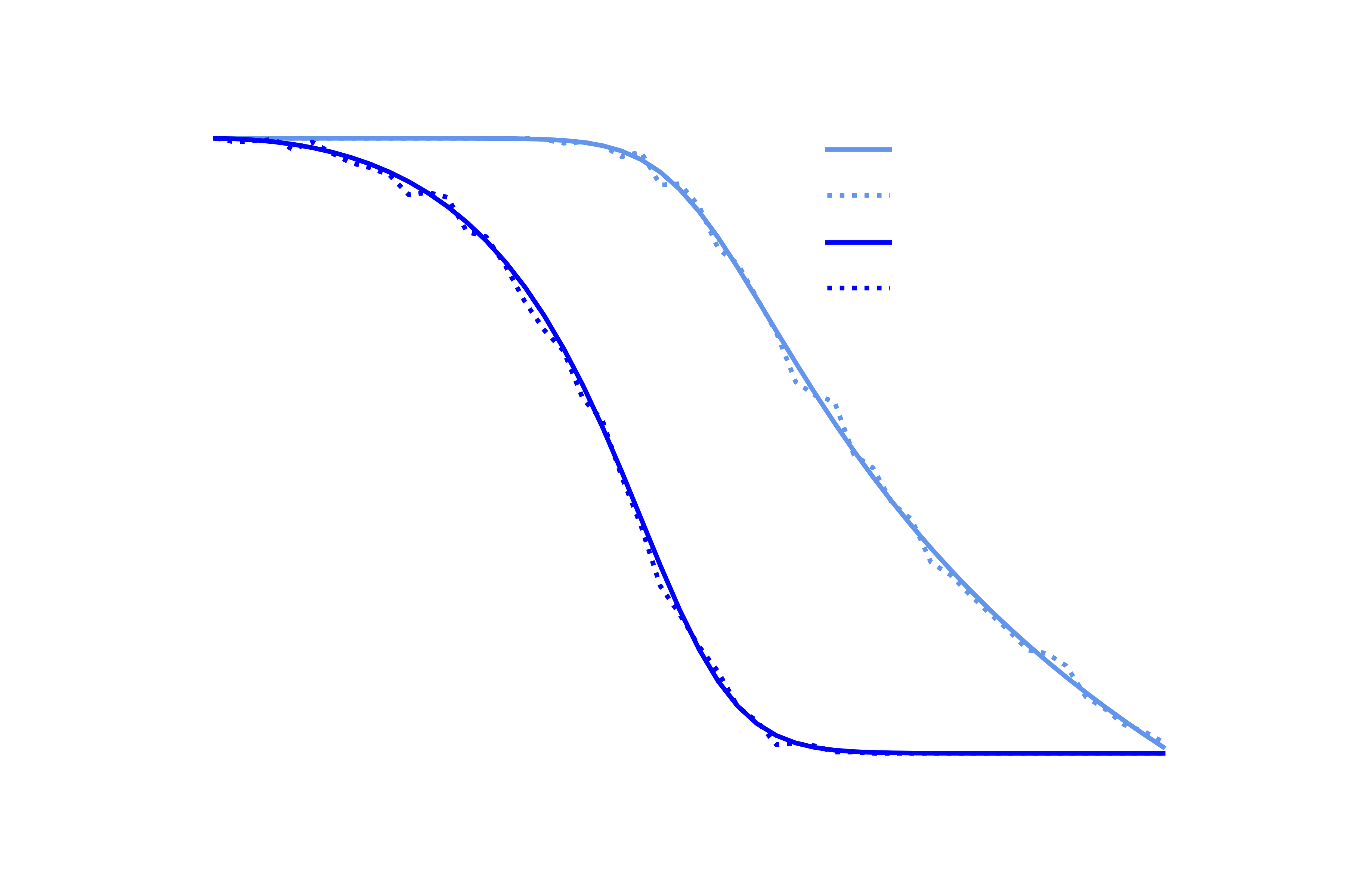
OK so now we have methods to calculate the probability of ruin both using simulation and analytically, let’s see how they compare. Below are plots of the probability of winning the game against the probability of winning a play $P$, for starting capital $C=\pounds 8$ and $C=\pounds 1$, using 500 simulated games. We can see that there is very good agreement between the two methods.

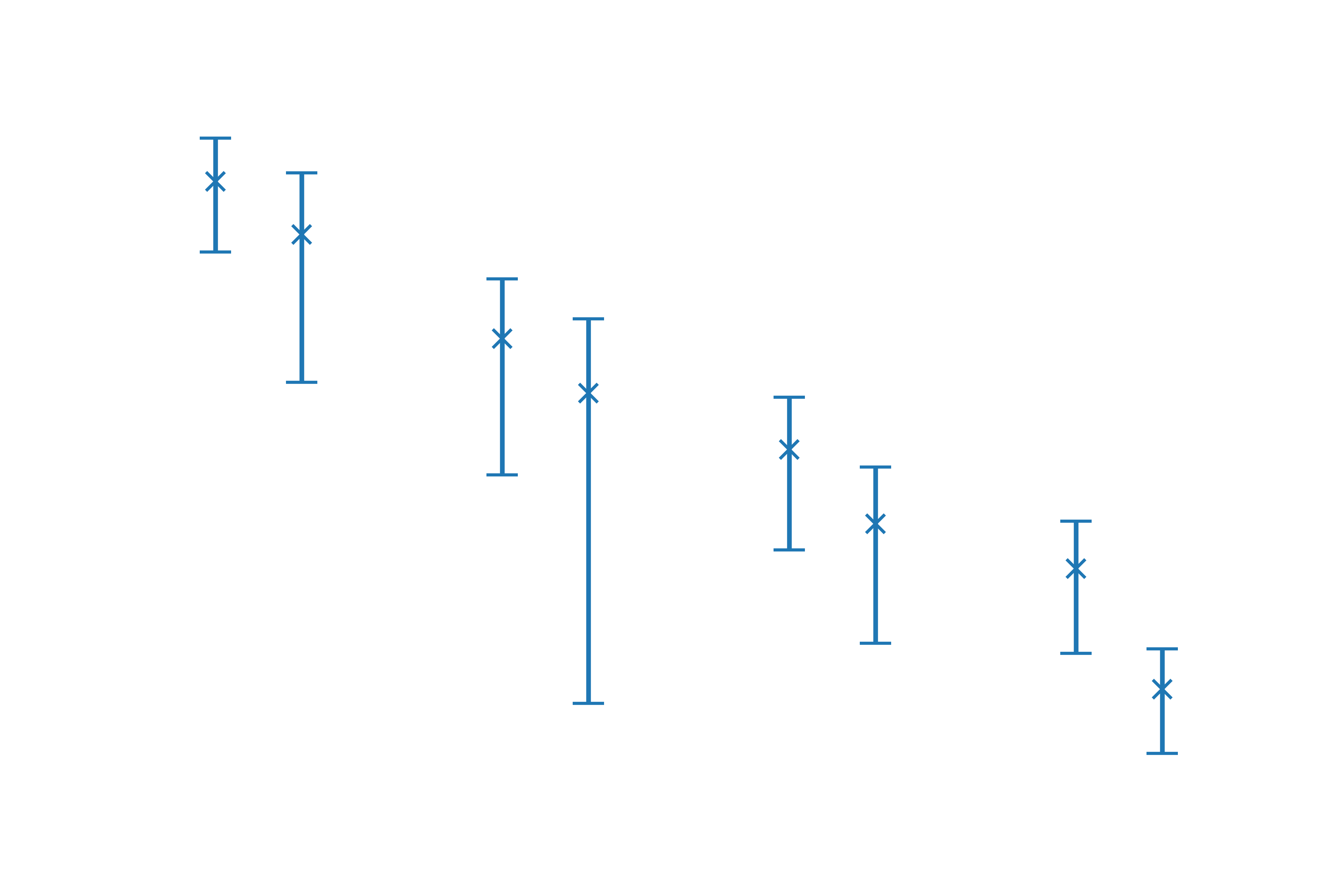
We can get a better idea about the error introduced by using the simulated method from the following plot of error against number of simulated games, with error bars computed from 5 repeats. The gradient of the graph is about 0.5 and since the axis are log scale this corresponds to the relationship $E\propto \frac{1}{\sqrt{N}}$, where $E$ is error and $N$ is number of games. This is consistent with the standard result for the error of a Monte Carlo estimator.

Conclusions⌗

I think the most important thing to consider when comparing the two solutions before we even think about errors, computation time etc, is simplicity. The code for the simulations took me less than 5 minutes to write. I spent about an hour trying to come up with an analytical solution with no luck, I then looked up the solution, and it took me quite a while longer to get my head round it. Even simple problems in probability can end up being analytically intractable, meaning no closed form solution can ever be found, let alone by me. For this reason Taleb is right to emphasize the power of the Monte Carlo engine, I hope this post has gone some way to illustrates it practical application.

Thanks for reading!