Maths problems
This is a list of maths problems (from textbooks, lecture notes etc.) that I have been looking at and have found interesting to solve.
6. Expectation maximization for mixture of linear experts.⌗
Source: Probabilistic machine learning: an introduction by Kevin P. Murphy, Ex. 11.6
Date: 2023-06-19
The EM algorithm for me is one of those things that I feel I should know back to front, since it’s a pretty foundational algorithm in probabilistic ML. Unfortunately though I’ve never actually used it explicitly in a model I have built, despite reading about it in various textbooks, so I never properly got to grips with it. If you feel the same way, then hopefully this question will help. It’s from the new Murphy book, which is a fantastic reference. So much for sticking to a problem a week, hopefully it won’t be such a long gap to the next one!
Problem
Derive the EM equations for fitting a mixture of linear regression experts.
Solution
We can fine the specification of the mixture of linear experts model in section 13.6.2.1 of the book. For input data $\{(x_n, y_n)\}^{N}_{n=1}$ with $x_n \in \mathbb{R}^D$ model consists of a set of $K$ linear models (called the experts), with weights $w_{k}\in\mathbb R^{D}$ with each linear model having a Gaussian likelihood, with noise variance $\sigma^2_k$. Additionally, we have a $K$-class logistic regression model, with weights $W\in\mathbb{R}^{K\times D}$, which outputs the probability that each expert is responsible for a particular data point. This model is written as,
\begin{align}
p(y|x_n,z=k,\theta)&=\mathcal{N}(y|w_{k}^{\mathsf{T}}x,\sigma_{k}^{2})\\\
p(z=k|x,\theta)&={\mathrm{Cat}}(z|{\mathrm{softmax}}_{k}(\mathrm{V}x)
\end{align}
where $\mathrm{Cat}$ is the categorical distribution and $\theta=(W, V, \{\sigma_k\}^{K}_{k=1})$ is our set of model parameters (in this case we assume $K$ is known, or selected by some other method like cross validation). The aim is to use EM to fit this model by finding $\theta$. Before getting into that, it’s perhaps helpful to look at the type of problem this model might be useful for.
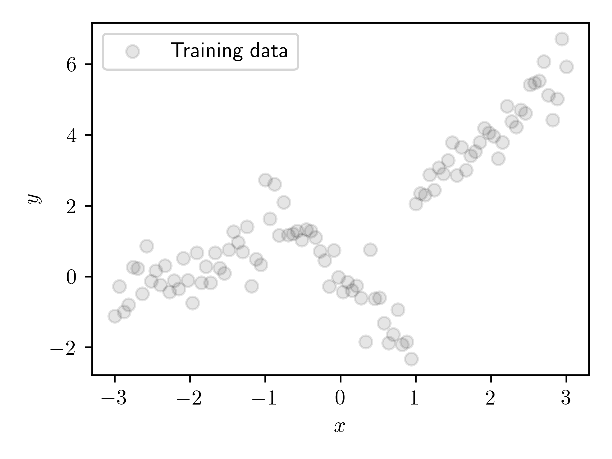
This is some data from a piecewise linear model, with 3 sections, with Gaussian noise added to it. We would hope that a mixture of linear experts model would be able to fit this data well, by assigning a different expert (i.e. linear model) to each of the distinct sections.
Now for inference. Recall that the point of the EM algorithm is to compute the maximum likelihood estimate of the model parameters, whilst marginalising out any latent variables. In this case the latent variables are the expert assignments for each data point, i.e. which expert is responsible for each data point. To do this, we alternate between two steps the E-step and the M-step, until we reach some sort of convergence:
- In the E-step, we compute the distribution of the latent variables (expert assignments) given the data and parameters, $p(z_n=k| y_n,x_n, \theta)$. In our case this is is tractable, if it’s not then you can use an approximating distribution, in which case the method becomes variational EM.
- In the M-step, we compute a quantity called the expected complete data log likelihood. This is the expected joint log probability of the data and latent variables, with respect to the distribution over the latent variables computed in the E-step, which we write as $\ell(\theta)=\sum_{n}\mathbb{E}_{q_{n}(z_{n})}\left[\log p(y_{n},z_{n}|\theta)\right]$ with $q(z_n)=p(z_n=k| y_n,x_n, \theta)$. We maximise this with respect to $\theta$, i.e compute $\theta^*=\mathrm{argmax}[l(\theta)]$. We then set $\theta=\theta^*$ and repeat the E-step.
We repeat this until the optimum of value in the M-step converges. For more info, see section 8.7 of the Murphy book. Now we can try to compute the required quantities for each step for the linear experts model.
We can compute the distribution over the latent variables given the data in the E-step using Bayes rule, $$ p(z_n=k| y_n,x_n, \theta) = \frac{p(y_n | z_n=k, x_n, \theta)p(z_n=k| x_n, \theta)}{p(y_n|x_n, \theta)} $$ where $p(y_n|x_n, \theta)=\sum^{K}_{k'=1} p(y_n | z_n=k', x_n, \theta)p(z_n=k'| x_n, \theta)$. This is tractable, we just combine the terms given in the specification of the model. Easy! Now for the M-step, which is slightly more involved.
For the M-step we need to compute $\sum_n\mathbb{E}_{q_{n}(z_{n})}\left[\log p(y_{n},z_{n}|\theta)\right]$ with $q_(z_n)=p(z_n=k| y_n,x_n, \theta)$. The log joint is given by,
\begin{align}
\log p(y_{n},z_{n}|\theta) &= \log p(y_{n}|z_{n},\theta)p(z_{n}|\theta) \\\
&= \log \prod_k\left[\mathcal{N}(y_n|w_{k}^{\mathsf{T}}x_n,\sigma_{k}^{2})\right]^{z_{nk}} + \log\prod_k\left[\frac{e^{v_{k}^\top x_n}}{\sum_{k'}e^{v_{k'}^\top x_n }}\right]^{z_{nk}} \\\
&=\sum_k {z_{nk}\log \left[\mathcal{N}(y|w_{k}^{\mathsf{T}}x,\sigma_{k}^{2})\right]} + \sum_k{z_{nk}}\log\left[\frac{e^{v_{k}^\top x_n}}{\sum_{k'}e^{v_{k'}^\top x_n }}\right]
\end{align}
where $z_{nk}$ is an indicator variable which is $1$ when $z_n=k$ and $0$ otherwise. We can the compute the M-step obejective as,
\begin{align}
\ell(\theta)&=\sum_n\mathbb{E}_{q_{n}(z_{n})}\left[\log p(y_{n},z_{n}|\theta)\right]\\\
&= \mathbb{E}_{q_{n}(z_{n})}\left[\sum_{nk} {z_{nk}\log \left[\mathcal{N}(y|w_{k}^{\mathsf{T}}x,\sigma_{k}^{2})\right]} + \sum_{nk}{z_{nk}}\log\left[\frac{e^{v_{k}^\top x_n}}{\sum_{k'}e^{v_{k'}^\top x_n }}\right]\right] \\\
&= \sum_{nk} {\mathbb{E}_{q_{n}(z_{n})}[z_{nk}]\log \left[\mathcal{N}(y|w_{k}^{\mathsf{T}}x,\sigma_{k}^{2})\right]} + \sum_{nk}{\mathbb{E}_{q_{n}(z_{n})}[z_{nk}]}\log\left[\frac{e^{v_{k}^\top x_n}}{\sum_{k'}e^{v_{k'}^\top x_n }}\right]
\end{align}
where $\mathbb{E}_{q_{n}(z_{n})}[z_{nk}]= p(z_n=k| y_n,x_n, \theta)$ are exactly the values computed in the E-step.
We are now able to compute $\ell(\theta)$, but we also need to optimise it. I think would be possible to compute the optimum with respect to the regression weights and variances exactly, using the formalism of weighted least squares, but if you’re lazy like me, you can just do simple gradient descent on the parameters. You’d have do this for the logistic weights anyway, since they can’t be computed in closed form, so it’s easier to just do this for everything.
Now we have both steps we can do inference. I implemented this using jax, which made the the optimisation for the M-step very easy. You can find the very shoddily written code in this gist.
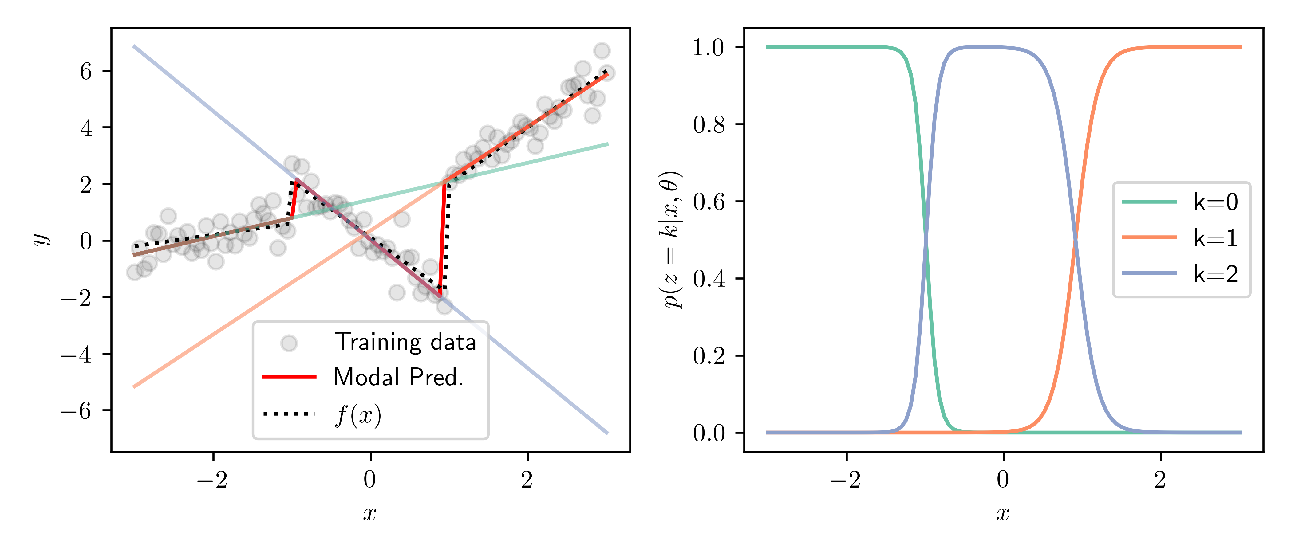
Above are the results after 20 EM iterations. The left panel shows the training data and true function, along with the predictions of each of the $K=3$ experts. Shown in red is the modal prediction, i.e. the prediction of the most likely expert for each point. The right panel shows the responsibilities of each expert for over the domain. We can see the transitions between experts nicely match the discontinuities in the piecewise function, and we are able to recover the true function well.
5. Distributions of quotients of uniform RVs.⌗
Source: Cut the knot by Bogomolny, Ex. 7.6
Date: 2023-04-20
This is a nice problem from the book “Cut the knot”, which is a compilation of probability riddles and brain teasers. I like the book because many of the problems are about intuitive reasoning, and don’t really involve that much technical knowledge of probability theory, so they can be fun to do with people who don’t have a formal maths background. Each problem can also generally be solved many different ways, so it’s fun to compare solutions.
Problem
Two numbers $X$ and $Y$ are randomly chosen from the interval $[0, 1]$. Let $r$ denote the quotient of the larger of the two by the smaller: $r = \frac{\max(X,Y)}{\min(X,Y)}$. Depending on the assumptions, there are three questions. For a given $k > 0$, what is the probability that $r ≥ k$
- if $X$ is uniformly distributed on $[0, 1]$ and $Y$ is uniformly distributed on $[X, 1]$?
- if $X$, $Y$ are jointly uniformly distributed on $\{(x, y) : 0 ≤ x ≤ y ≤ 1\}$?
- if $X$ and $Y$ are uniformly and independently distributed on [0, 1]?
Solution
We’re given that $X\sim U(0, 1)$ and that $Y|X\sim U(X, 1)$, this implies that the variables have the densities
\begin{align}
p(x)&=1 \quad \forall \quad x\in[0, 1] \\\
p(y|x)&=\frac{1}{1-x} \quad \forall \quad y\in[x, 1]
\end{align}
which implies that the variables have the joint density given by
$$
p(x, y) = p(x)p(y|x)= \frac{1}{1-x}.
$$
Now let’s have a think about how to compute the require probability $\mathbb{P}(r\geq k)$. First, it is clear that in this case $Y\geq X$, so $r\geq1$ which implies $\mathbb{P}(r\geq k)=1$ when $k<1$. The fact that $Y\geq X$ also implies that $r = \frac{\max(X,Y)}{\min(X,Y)}=\frac{Y}{X}$. The key thing to realize here is that we can equivalently write $\mathbb{P}(r\geq k)$ as $\mathbb{P}(\frac{Y}{X}\geq k)=\mathbb{P}(Y\geq kX)$.
We actually now have all the parts we need to solve the question, but realizing this is a little easier with a picture. The diagram below shows all the information we have. The variables $x$ and $y$ are shown on each axis, with the shaded region showing the probability density of different $(x,y)$ pairs. Notice that the lower triangle is unshaded since we know $y>x$. Also plotted on the diagram is the line $y=kx$.
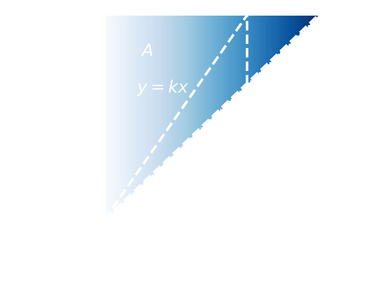
What we want to know is the probability that $(x,y)$ lies in the region $A$, i.e the region bounded by $0\leq y \leq 1, y\geq kx$. To do this we need to integrate the joint density over this region. This probability is given by
\begin{align}
\mathbb{P}(r\geq k) &= \int^{1/k}_{0} \int^{1}_{kx}p(x,y)dydx\\\
&= \int^{1/k}_{0} \int^{1}_{kx} \frac{1}{1-x}dydx \\\
&= \int^{1/k}_{0} \frac{1-kx}{1-x}dx \\\
&= 1 + (k-1)\log\left(\frac{k-1}{k}\right)
\end{align}
Part 1 solved!
Now we have this setup the answers for the next two parts are actually quite simple. For part 2, we have the exact same setup, only now we are given that the $X,Y$ are jointly uniform over the region $0\leq x\leq y \leq 1$. The diagram would look exactly the same, but with the shading being uniform over the region. The joint density is now $p(x,y)=2$ (since the area of the region is $1/2$), so
\begin{align}
\mathbb{P}(r\geq k) &= \int^{1/k}_{0} \int^{1}_{kx}p(x,y)dydx\\\
&= 2\int^{1/k}_{0} \int^{1}_{kx} dydx \\\
&= \frac{1}{k}
\end{align}
Now for the final part, we can use the symmetry of the problem to get the answer easily. When $Y>X$ we have the same setup as above, and when $X>Y$ we have the region $0\leq x\leq 1, y\leq\frac{x}{k}$, which is the mirror image of the region from part 2, reflected in $y=x$. We sum these regions to get the answer. Not that the density is now $p(x,y)=1$, so we get that $$ \mathbb{P}(r\geq k) = \frac{1}{2k} + \frac{1}{2k} = \frac{1}{k} $$
4. Mercer theorem measure and RKHS norm.⌗
Source: Gaussian Processes for Machine Learning by Rasmussen and Williams, Ex. 6.7.1
Date: 2023-04-12
This problem from the GPML book relates to the effect of the choice of measure when using Mercer’s theorem to compute kernel eigenfunctions on the resulting norm in the RKHS induced by that kernel. In the problem we show that in the finite dimensional case (this also applies in the $\infty$ dimensions case but it is then harder to show), the RKHS norm is independent of the measure chosen. This is interesting to me because when first learning about Mercer’s theorem, I was confused by how the measure the eigenfunctions are computed w.r.t is chosen when using the theorem in practice. This question shows that in for some important applications, the measure doesn’t matter.
Problem
We motivate the fact that the RKHS norm does not depend on the density $p(x)$ using a finite-dimensional analogue. Consider the n-dimensional vector $\mathbf f$, and let the $n \times n$ matrix $\Phi$ be comprised of non-colinear columns $\phi_1,\dots, \phi_n$. Then $\mathbf f$ can be expressed as a linear combination of these basis vectors $\mathbf f = \sum^n_{i=1} c_i\phi_i = \Phi \mathbf c$ for some coefficients $\{c_i\}$. Let the $\phi$s be eigenvectors of the covariance matrix $K$ w.r.t. a diagonal matrix $P$ with non-negative entries, so that $KP \Phi = \Phi\Lambda$, where $\Lambda$ is a diagonal matrix containing the eigenvalues. Note that $\Phi^\top P\Phi = I$. Show that $\sum^n_{i=1}c^2_i/\lambda_i=\mathbf c^\top\Lambda^{-1}\mathbf c=\mathbf f^\top K^{-1} \mathbf f$, and thus observe that $\mathbf f^\top K^{-1} \mathbf f$ can be expressed as $ \mathbf c^\top\Lambda\mathbf c$ for any valid $P$ and corresponding $\Phi$. (Note the matrix $P$ here represents the measure.)
Solution
This solution is a bit strange as I got stuck and this is the only way I could think to do it, I am sure there is a better way. First using that $\Phi^\top P\Phi = I$ we can see that,
$$
KP\Phi=\Phi\Lambda \implies \Phi^\top PKP\Phi=\Lambda.
$$
We can then write
\begin{align}
\mathbf c^\top \Lambda^{-1} \mathbf c &= \mathbf c^\top (\Phi^\top PKP\Phi)^{-1} \mathbf c \\\
&= \mathbf c^\top \Phi^{-1}P^{-1}K^{-1}P^{-1}\Phi^{-\top} \mathbf c \\\
&= \mathbf c^\top \Phi^\top P P^{-1}K^{-1}P^{-1} P \Phi \mathbf c \\\
&=\mathbf f^{\top} K^{-1} \mathbf f
\end{align}
as required, where on the second to last line we have twice used the fact that $\Phi^{-1}=\Phi^\top P$.
3. Converting state misalignment in probabilistic numeric ODE solver to SDE.⌗
Source: Probabilistic Numerics by Henning, Osborne and Kersting, Ex. 38.1
Date: 2023-04-03
It is only the third week and I have already failed to manage my goal of posting one solution per week, not a good sign for the future… In my defense, I was busy last week attending the Probabilistic Numerics Spring School, at which I learned lots about probabilistic ODE solvers, on which this weeks late question is based.
Probabilistic ODE solvers work by placing a Markovian GP prior (usually the $q$-times integrated Wiener process) over the solution, given this prior, we then condition on the fact samples of this GP must solve the ODE at a given set of time steps, that is to say the derivatives of the GP prior must match the derivative function of the ODE. We can infer the solution to the ODE by using filtering and smoothing techniques from signal processing. In this question, the task is to form an SDE for the state misalignment, i.e the difference between the derivatives of the prior and the ODE derivative function. It is interesting to note that we can also condition on other properties of the system, for example, conditioning on energy conservation in a Hamiltonian system leads to a symplectic solver, see here for details. The whole idea is fascinating and deserves a look if you have never come across it.
Problem
We take our prior to be the SDE $$ dX(t)=FX(t)dt + Ld\omega, $$ with $X \in\mathbb{R}^{D}$, $F,L\in\mathbb{R}^{D \times D}$ and $d\omega \in\mathbb{R}^{D}$ being an increment of the Wiener process with diffusion $Q\in\mathbb{R}^{D \times D}$. We also have two projection matrices which allow us to obtain the parts of the SDE prior that represent ODE state, and ODE state derivative, $$ \mathbf x(t) = H_0X(t), \qquad \mathbf x'(t) = HX(t). $$ with $H,H_0\in\mathbb{R}^{d \times D}$ where $d$ is our ODE dimension. The state misalignment is given by $$ Z(t) = \phi(X(t))=HX(t) - f(H_0X(t)). $$ where $f: \mathbb{R}^D \mapsto \mathbb{R}^D$ is our ODE derivative function and $Z(t)\in\mathbb{R}^d$ is called the observation process, and is given by another SDE. Our task is to find an expression for this SDE and state under which conditions it is Gaussian process.
Solution
The Itô formula for transformations of SDEs by scalar funtion $g(X(t))$ is given by $$ dg = (\nabla g) dX + \frac{1}{2}\operatorname{tr}[(\nabla^\top \nabla g) dXdX^\top]. $$
(Note: here I have used the gradient as row vector) We need to use this to compute the the transformation represented by the state misalignment, which is a vector function. Fortunately, the Itô formula applies to each componnt, so $$ d\phi_i = (\nabla \phi_i) dX + \frac{1}{2}\operatorname{tr}[(\nabla^\top \nabla \phi_i) dXdX^\top]. $$ with $$ \phi_i = \sum_j H_{i,j} X_j + f_i(H_0 X). $$ We now need to compute the Jacobian and the Hessian given in the formula. This took me a long time as my vector calculus is a little rusty, and I am not 100% sure I have the correct answer but I got them to be, $$ \nabla \phi_i = H_{i,-} + \nabla f_i(H_0 X)H_0^\top $$ where $\nabla f_i$ is the Jacobian of $f$ for output $i$ and $H_{i,-}\in \mathbb{R}^D$ is the $i$-th column of $H$, and for the Hessain,
$$
\nabla^\top\nabla \phi_i = H_0[\nabla^\top\nabla f_i(H_0 X)]H_0^\top
$$
where $\nabla^\top\nabla f_i$ is the Hessian of $f$ for output $i$. We also need that
\begin{align}
dXdX^\top &= (FX(t)dt + Ld\omega)(FX(t)dt + Ld\omega)^\top \\\
&=LQL^\top dt
\end{align}
where we use the combination rules for mixed differentials given in the Itô formula. Subbing all this into the formula and collecting terms, we obtain the SDEs,
\begin{align}
d\phi_i = &\left(H_{i,-}FX(t) + \nabla f_i(H_0 X)H_0^\top X(t) + \frac{1}{2}\operatorname{tr}(H_0[\nabla^\top\nabla f_i(H_0 X)]H_0^\top LQL^\top)\right)dt \\\
&+ (H_{i,-}+ \nabla f_i(H_0 X)H_0^\top)Ld\omega
\end{align}
which can then be simulated to give the observation process. This SDE will be a GP when $f$ is linear, since GP representations of SDEs do not have multiplicative noise (see Särkkä and Solin book, 6.1), so we require that the gradient of $f$ be independent of $X$ which is only true when we have a linear derivative function.
2. Relationship between the Frobenius norm and singular values in SVD.⌗
Source: ChatGPT, Mathematics for Machine Learning by Deisenroth, Faisal and Ong
Date: 2023-03-22
Problem
Note: I was brushing up on my SVD using the brilliant “Mathematics for Machine Learning” book, but the exercises listed in the book for SVD were a bit basic, so I decided to try use ChatGPT to generate a question. The problem below is what came out, quite impressive, although there were quite a few errors in the question that I had to fix (e.g the dimensionalities of the matrices).
Let $A$ be an $m \times n$ with $m\geq n$ matrix with rank $r$, and let its singular value decomposition (SVD) be given by $A = U \Sigma V^T$, where $U$ is an $m \times m$ orthonormal matrix, $\Sigma$ is an $m \times n$ diagonal matrix with non-negative entries $\sigma_1 \geq \sigma_2 \geq \dots \geq \sigma_n > 0$, and $V$ is an $n \times n$ orthonormal matrix. Show that the Frobenius norm of $A$ is equal to the square root of the sum of the squares of the singular values.
Solution
The Frobenius norm is given by,
$$
||A||^2_F = \sum_{i,j}A^2_{i,j}
$$
which we can equivalently write (it is not so hard to show this) as
$$
||A||^2_F = \operatorname{tr}(A^\top A).
$$
Subbing in the SVD representation of $A$, we get
\begin{align}
\operatorname{tr}(A^\top A) &= \operatorname{tr}\left( (U\Sigma V^\top)^\top(U\Sigma V^\top)\right)\\\
&= \operatorname{tr}\left(V\Sigma^\top U^\top U\Sigma V^\top\right) \\\
&= \operatorname{tr}\left(V\Sigma^\top \Sigma V^\top\right).
\end{align}
We can see by inspection that $\Sigma^\top\Sigma = \operatorname{diag}(\sigma^2_1, \dots, \sigma^2_n)=\Lambda$. This implies that
$$
[V\Lambda V^\top]_{ii} = \sigma_i^2\mathbf{v}^\top_i\mathbf{v}_i = \sigma_i^2,
$$
where $\mathbf{v}_i$ is column $i$ of $V$ and the second equality follows from the othonormality of $V$. Putting it all together we get that
$$
||A||^2_F = \operatorname{tr}(A^\top A) = \sum_i \sigma_i^2,
$$
as required.
1. Winners curse in Bayesian optimisation.⌗
Source: Probabilistic Numerics by Henning, Osborne and Kersting, Ex. 32.2
Date: 2023-03-14
Problem
Take an objective function $f(x)$ with GP prior and i.i.d. Gaussian noise with variance $\sigma^2$, so $y_i = f(x_i) + \epsilon_i$ with $\epsilon_i \sim \mathcal{N}(0, \sigma^2)$. Assume two locations $x_1, x_2$ are sufficiently separated that their function values $f(x_1)$ and $f(x_2)$ are independent. Compute the posterior $p(\epsilon_1-\epsilon_2|y_1, y_2)$ and use it to justify that the expected improvement in Bayesian optimisation suffers winners curse for a noisy objective. The winners curse says that for noisy optimisation problems, the lowest value is also likely the most noisy.
Solution
First we need to compute $p(\epsilon_i| y_i)$, which we can do using Bayes rule,
$$
p(\epsilon_i| y_i) = \frac{p(y_i| \epsilon_i)p(\epsilon_i)}{p(y_i)}
$$
we have that $p(\epsilon_i) = \mathcal{N}(\epsilon_i; 0, \sigma^2)$, and that $p(y_i| \epsilon_i) = \mathcal{N}(y_i; \epsilon_i, \sigma_f^2)$ where we have assumed that the prior over $f$ has 0 mean, and variance $\sigma_f^2$. So we have,
$$
p(\epsilon_i| y_i) \propto \mathcal{N}(y_i; \epsilon_i, \sigma_f^2)\mathcal{N}(\epsilon_i; 0, \sigma^2)
$$
which we can identify as a product of Gaussian PDFs. This results in another Gaussian PDF, see e.g these notes,
$$
p(\epsilon_i| y_i) = \mathcal{N}(\epsilon_i; \mu_{\epsilon_i}, \sigma^2_{\epsilon_i}),
$$
where
\begin{align}
\mu_{\epsilon_i} &= \frac{y_i\sigma^2}{\sigma^2 + \sigma_f^2}, \\\
\sigma^2_{\epsilon_i} &= \frac{\sigma_f^2\sigma^2}{\sigma^2 + \sigma_f^2}.
\end{align}
We can see here that the variance is independent of data. Now we have computed the posterior of the noise given the data, we can compute the posterior of the difference between the noises given the data. Since the function values at the input points are independent then the posterior over the difference is just the difference of independent Gaussian random variables, in which case we simply subtract the means and sum the variances, to give
$$
p(\epsilon_1 - \epsilon_2=\Delta| y_1, y_2) = \mathcal{N}\left(\Delta; \frac{\sigma^2}{\sigma^2 + \sigma_f^2}(y_1-y_2), 2\sigma^2_{\epsilon}\right).
$$
The key point here is that the mean of this distribution depends on the difference between the data values. So
$$
y_1>y_2 \implies \mathbb{E}[\epsilon_1 - \epsilon_2]> 0 \implies \mathbb{E}[\epsilon_1] > \mathbb{E}[\epsilon_2].
$$
If we assume that the values are lower that the prior mean (i.e. 0), which is to be expected, then we expect the noise for the lower point to be a larger (absolute) value. This is the winners curse described in the book.