(Note: This series of posts is closely related to and inspired by this paper from Miles Cranmer, Sam Greydanus, Stephan Hoyer and others. To accompany the paper they also wrote a brilliant blog post about the work which I would encourage you to read)
I really enjoy Lagrangian mechanics, in fact, I would go so far as to say that studying it was one of the best parts of my physics degree. We will get into the reasons for this shortly, but needless to say, when I heard that Lagrangians were being used with neural networks to learn physics I could not have clicked the arXiv link faster. In this series of posts I will give a brief introduction to what Lagrangian mechanics is all about, why the concepts are so important in physics, and how we can use them to solve a cool problem involving both a pendulum and a spring at once (!). We’ll then see how we can use PyTorch to save ourselves the effort of calculating a load of derivatives by hand. Finally we’ll tie it all together to learn a Lagrangian from some data using a neural network, and see how we get superior performance by making the model aware of the physics of the situation. Lots to do, so let’s get started!
What is a Lagrangian?
To solve a problem in classical mechanics you generally need to find the equations of motion of the system in question. These equations, when solved, completely determine the trajectories of the constituent parts of the system. One extremely simple example is a particle in free fall which has the equation of motion . The Lagrangian (almost always written as ) is a special function that contains all the dynamics of the system, which can be used to find the equations of motion in a relatively simple way. is a function of the generalised coordinates describing our system, denoted and their corresponding time derivatives 1 2. One really useful aspect of Lagrangian mechanics is that as long as the ’s totally specify our system, they can be pretty much anything we want (e.g. positions, angles, lengths) this is very powerful and is not true in Newtonian mechanics.
Problems with Newtonian Mechanics
You may be wondering why we need to do all this complicated stuff with Lagrangians when Newton’s laws, which most people learn in school, can in theory solve every problem possible in classical mechanics. There are a number of interesting reasons for this which are discussed extensively elsewhere, the most relevant here is the fact that it is often very difficult to actually write down Newton’s laws for a given system. In Newtonian mechanics we consider the action of force vectors on particles. Because all the forces in a problem must be written explicitly, systems that have complex constraints, e.g. double pendulum, can be very hard to deal with. For rotational systems, it can be difficult to exploit symmetry of because sets of angles aren’t really vectors.
Finding the equations of motion from involves using Hamilton’s principle of least action, which is stated in loose terms below:
“The trajectory followed by a system is the one with the smallest action”
The action, , of a trajectory is the time averaged value of the Lagrangian along it. More formally it is the functional,
Using two classic physicists tricks, reverse integration by parts and a first order Taylor expansion, you can figure out that systems obeying Hamilton’s principle must have,
for each . These are known as the Euler-Lagrange equations. Without a concrete example, this all seems very abstract and confusing, but the upshot is if we know then we can work out the equations of motion. Just one final piece of the puzzle before we can actually work stuff out, how do we find ? It turns out that in classical, non relativistic mechanics it is given by the simple expression,
where is the kinetic energy of the system, and is the potential energy. It is almost always easier to think of the different energies in a system than it is to resolve forces, which is why Lagrangian mechanics is so powerful.
The Real Power of Lagrangians
Although Lagrangians are an important tool in classical mechanics, they actually play a much more pivotal role in the fundamental physics of the Universe. The Standard Model, which describes all fundamental particles (e.g photons, electrons, quarks) is specified as a Lagrangian. Lagrangians can be constructed in such a way that their value does not change when changing reference frames, which means they can be made consistent with Einstein’s theory of special relativity. Also Noether’s theorem means that conservation laws (e.g. for momentum, charge), can be incorporated into the Lagrangian formalism in a very natural way.
A Fun Example!
Ok so now we have the theory bit out the way let’s have a go at actually using a Lagrangian in practice. The problem we are going to consider is a spring pendulum, this is really what it says on the tin, a spring with a mass attached that can freely swing about some fixed point. The setup is shown in the handy diagram below.
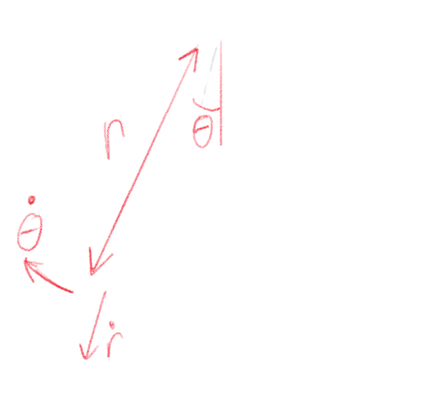
A handy diagram.
It is clear that there are 4 generalised coordinates which fully describe the system: , the angle the spring makes with the vertical, , the length of the pendulum, and their corresponding time derivatives, and . Having identified these it’s pretty easy to think of all the kinetic and potential in the energies in the system, try to think of them and then have a look at the list below to see if you got it correct:
-
Linear kinetic energy, , from by the movement of the mass in the direction of the spring.
-
Rotational kinetic energy, , from the rotation of the mass about the fixed point the spring is attached to.
-
Mechanical potential energy, , from the compression and extension of the spring.
-
Gravitational potential energy, , from the changing height of the mass.
1-3 are given by standard formulas, for example Hooke’s law for 3, and can be written down straight away. 4 just involves using a bit of trigonometry to work out the vertical height of the spring in terms of , then applying the standard formula for a uniform gravitational field. Each formula is shown in the table below, where m is the mass, is the length of the unextended spring and is the gravitational constant:
| Energy | Formula |
|---|---|
Taking , we can now finally write down the full Lagrangian as,
So to find the equations of motion from here we need to apply the Euler-Lagrange equations, which involves calculating the partial derivatives with respect to each independent variable, this is a bit tedious but not too bad,
The final step is to plug these into the Euler-Lagrange equations, and apply the total time derivative, then rearrange to get the following 2 equations of motion:
Mission complete! Unfortunately because these are coupled non-linear differential equations, they can’t be solved analytically (by me at least), so we need to use a numerical solver. Solving differential equations numerically is obviously a huge subject, so I won’t go into any detail here, but it is currently quite a hot topic in ML research, see for example this paper. To solve our equations of motion we can use the handy odeint function from scipy.
Spring pendulums in motion.
Above is a gif of 3 pendulums with different initial conditions 3. The motion is pretty much what we would expect, so everything seems to be working! Everything we have done so far is taught in a standard undergraduate physics course, so now we have the basics down let’s see how we can involve the ML.
Bringing in PyTorch
Disclaimer: Before this project I had never used PyTorch, in fact part of the reason for doing the project was to get familiar with using it. For this reason it is likely that some of my code is bad practice/wrong. If you spot any mistakes, please let me know, thanks!
In this section we’re going to see how we can use the autograd functionality in PyTorch to automatically determine the equations of motion from our Lagrangian. To do this we need to think a bit about what the equations of motion actually are. First let’s put all our independent generalised coordinates into a vector, . The value of completely specifies the state of our system. The equations of motion tell us the dynamics of our system, i.e. how the state evolves forward in time. They can be written concisely as,
if we know we know the dynamics of the system. We already have the top 2 components of , since they are both generalised coordinates, so all we need to do is find the bottom 2. For clarity lets write the and the bottom 2 as . The challenge then is to find . Using this notation we can write the Euler-Lagrange equations as,4
We can then explicitly apply the the total time derivative to get,
This derivative confused me a bit when I first read the original paper, so may it be worth showing a few more steps. Feel free to skip this mini section if you’re already happy with it!
Derivatve Derivation
When computing the total derivative, we need to remember to take all the time dependence into account, this means using the chain rule on everything the Lagrangian depends on. We are trying to compute,
For simplicity let’s just work out the top component of this, applying the chain rule to incorporate all the time dependence,
Hopefully it is clear that if we replace, and so on, this would be the top component of the vector derivative, having multiplied everything out correctly.
The final step then is to do a bit of matrix algebra to get alone, we end up with,
Now we have alone we have a clear recipe for solving the system given an arbitrary differentiable Lagrangian. We just have to plug it into the equation above, work it through, then we have which we can use in a numerical differential equation solver to make some nice gifs. This expression is also helpful because it works for any number of generalised coordinates. This expression is really important when it comes to actually incorporating the neural network effectively, but we will get to that later.
Let’s write some code so that given a Lagrangian, we can automatically determine the equations of motion without having to go through all the derivatives by hand. Since PyTorch now has functions to calculate the Hessian and Jacobian, this is actually reasonably easy. The following function, returns for a given and state :
import torch
from torch.autograd.functional import jacobian, hessian

def get_xt(L, x):

    n = x.shape[0]//2 # Get number of generalised coords
    xv = torch.autograd.Variable(x, requires_grad=True)
    y, yt = torch.split(xv, 2, dim=0)

    # The hessian/jacobian are calculated w.r.t all variables in xv
    # so select only relevant parts using slices
    A = torch.inverse(hessian(L, xv, create_graph=True)[n:, n:])
    B = jacobian(L, xv, create_graph=True)[:n]
    C = hessian(L, xv, create_graph=True)[n:, :n]

    ytt = A @ (B - C @ yt)

    xt = torch.cat([yt, torch.squeeze(ytt)])

    return xt
To check it’s working correctly let’s test it on the spring pendulum, and use the same initial conditions in the equations we calculated by hand, then we can compare the trajectories and see if they are the same.
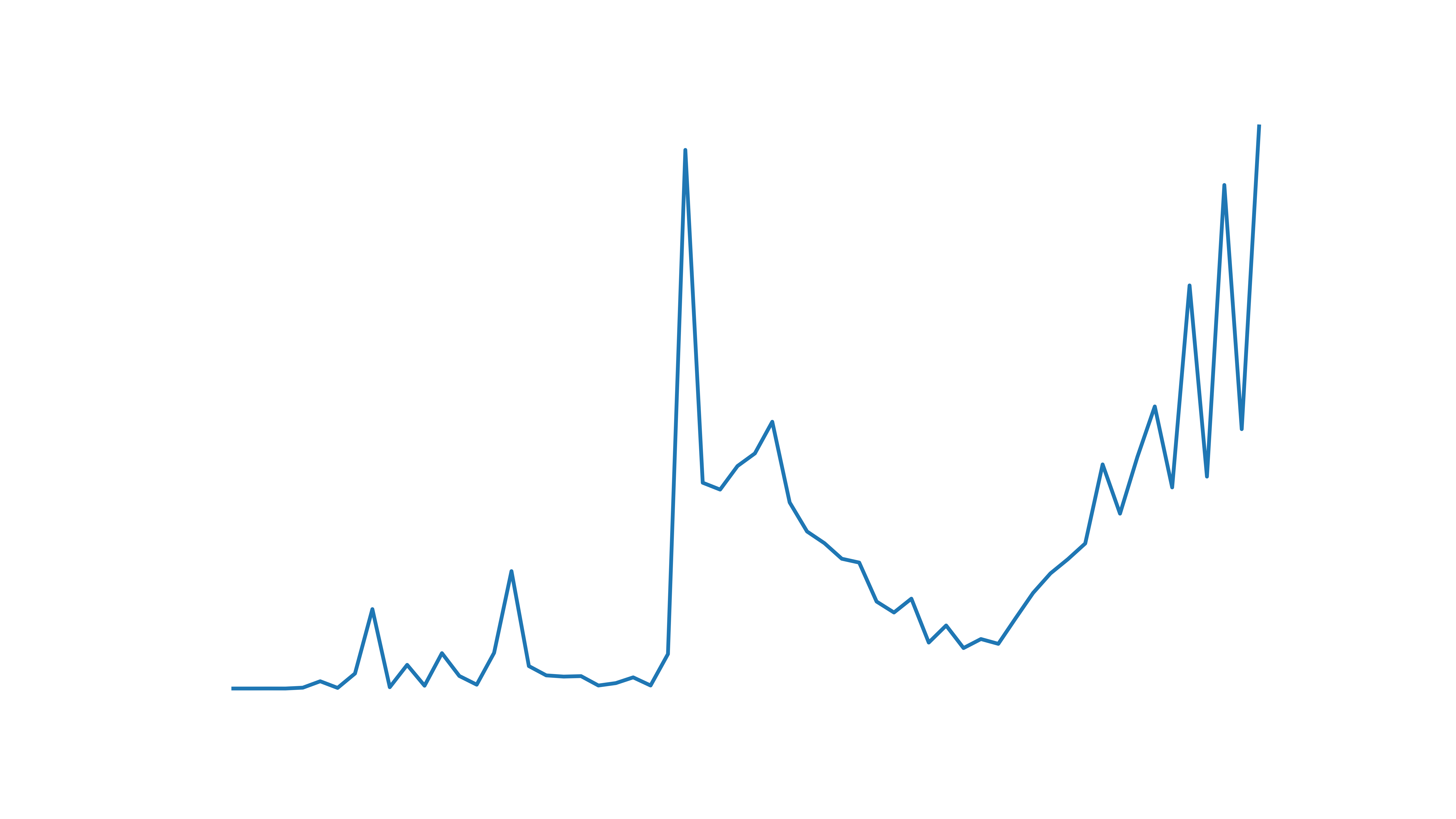
Mean square difference between components of each method, with increasing time.
At first glance this looks pretty bad, but the axis is y axis is at a scale , so the PyTorch method is giving almost exactly the same trajectory. Cool!
So where’s the ML?
We’ve done lots of physics so far, but where does the ML come in? Well the good news is that we now have all the ground work out of the way, and we are ready to dive into Lagrangian Neural Networks. In post #2 we will get straight into implementing LNNs in PyTorch, given the knowledge we now have, this should be a relatively simple task.
Let’s just recap a bit and think why we are doing all this in the first place. Here I have used an example of a mechanical system with a known Lagrangian, what if we want to determine the dynamics of a system which is known to obey the laws of classical mechanics, but the Lagrangian is not known? One option is to learn from data. As we discussed earlier all we need to determine the dynamics is the function . So why did we even need to bother with all this Lagrangian stuff? Why not just replace with a neural network, and learn it straight from the data? We could do this, and it is possible that with a large enough model we might get good results, but we can do much better by making the model aware of the physics of the situation. If instead we parameterise with a neural network, and then use our equation for to determine , then the Euler-Lagrange equations are included as constraints in the model. This means we have a neural network that is aware of Hamilton’s least action principle! Because the model is physics aware, we should get significantly better results from a model with fewer parameters. LNNs are a cool example of using physics knowledge to introduce inductive bias into an ML model. Another nice example of this from a totally different area of ML, Bayesian non-parametrics, are Latent Force Models, which may be the subject of a future post.
If you got this far thanks for reading, and hopefully you can join me for part #2 shortly!
-
We treat and as independent variables, this can be really confusing at first. You can get an intuitive feel for why this might true if you think about the fact you need to know both the position and velocity of a particle to fully determine it’s future trajectory. ↩︎
-
can also depend explicitly on time, which results in energy not being conserved, but we will not consider that case here. ↩︎
-
To create the gif I made plots with matplotlib, and then used this brilliant package to animate. ↩︎
-
As I mentioned before this derivation closely follows that in the Lagrangian Neural Networks paper, so all credit to the authors for it. ↩︎